Processing toolbox qgis как открыть

The QGIS Commander¶

Processing includes a practical tool that allows you to run algorithms without having to use the toolbox, but just by typing the name of the algorithm you want to run.

This tool is known as the QGIS commander, and it is just a simple text box with autocompletion where you type the command you want to run.

The QGIS Commander

The Commander is started from the Processing menu or, more practically, by pressing Shift + Ctrl + M (you can change that default keyboard shortcut in the QGIS configuration if you prefer a different one). To close it, just press ESC . Apart from executing Processing algorithms, the Commander gives you access to most of the functionality in QGIS, which means that it gives you a practical and efficient way of running QGIS tasks and allows you to control QGIS with reduced usage of buttons and menus.

Moreover, the Commander is configurable, so you can add your custom commands and have them just a few keystrokes away, making it a powerful tool to help you become more productive in your daily work with QGIS.

Доступные команды¶

The commands available in the Commander fall in the following categories:

• Processing algorithms. These are shown as Processing algorithm: .
• Menu items. These are shown as Menu item: . All menus items available from the QGIS interface are available, even if they are included in a submenu.
• Python functions. You can create short Python functions that will be then included in the list of available commands. They are shown as Function: .

To run any of the above, just start typing and then select the corresponding element from the list of available commands that appears after filtering the whole list of commands with the text you have entered.

In the case of calling a Python function, you can select the entry in the list, which is prefixed by Function: (for instance, Function: removeall ), or just directly type the function name ( removeall in the previous example). There is no need to add brackets after the function name.

Создание пользовательских функций¶

Custom functions are added by entering the corresponding Python code in the commands.py file that is found in the .qgis2/processing/commander directory in your user folder. It is just a simple Python file where you can add the functions that you need.

The file is created with a few example functions the first time you open the Commander. If you haven’t launched the Commander yet, you can create the file yourself. To edit the commands file, use your favourite text editor. You can also use a built-in editor by calling the edit command from the Commander. It will open the editor with the commands file, and you can edit it directly and then save your changes.

Например, можно добавить такую функцию для удаления всех слоёв:

from qgis.gui import * def removeall(): mapreg = QgsMapLayerRegistry.instance() mapreg.removeAllMapLayers() 

Once you have added the function, it will be available in the Commander, and you can invoke it by typing removeall . There is no need to do anything apart from writing the function itself.

Functions can receive parameters. Add *args to your function definition to receive arguments. When calling the function from the Commander, parameters have to be passed separated by spaces.

Вот пример функции, загружающей слой. В качестве параметра ей передаётся имя файла, который необходимо открыть.

import processing def load(*args): processing.load(args[0]) 

If you want to load the layer in ;file: /home/myuser/points.shp , type in the Commander text box:

load /home/myuser/points.shp 

QGIS: начало работы¶

Quantum GIS (QGIS) — это дружественная к пользователю настольная ГИС с открытым исходным кодом, позволяющая отображать, редактировать и анализировать данные, управлять ими, а также создавать печатные карты.

Этот документ описывает, как:

• обновить существующий проект QGIS;
• создать новый проект QGIS с простым векторным слоем.

Редактирование проекта QGIS¶

1. Нажмите Desktop ‣ Desktop GIS ‣ Quantum GIS .
2. Выберите в меню File ‣ Open Project. .
3. Укажите файл QGIS-NaturalEarth-Example.qgs и нажмите Open .
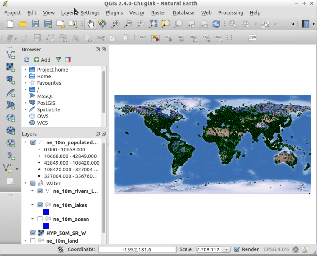
   • Вы должны увидеть карту мира.
4. В списке слоёв установите галку напротив 10m_populated_places_simple
   • Отобразятся города:
5. Дважды щёлкните на 10m_rivers_lake_centerlines в списке слоёв.
6. Измените цвет в Outline Options на другой оттенок голубого.
7. Нажмите OK .
   • Реки должны отобразиться другим цветом.

Создание нового проекта QGIS¶

1. Выберите File ‣ New Project .
2. Нажмите Layer ‣ Add Vector Layer. .
3. Перейдите к набору данных /home/user/data/natural_earth/10m_admin_0_countries.shp .
4. Нажмите Open .
   • Вы должны увидеть границы стран мира.

Подключение к пространственной базе данных PostGIS¶

1. Выберите File ‣ New Project .
2. Выберите Layer ‣ Add PostGIS Layers. .
   • Доступны две базы данных Natural Earth и OpenStreetMap.
3. Выберите базу данных OpenStreetMap и нажмите Connect .
   • Появится список таблиц базы данных.
4. Выберите planet_osm_roads и нажмите Add .
   • Более подробное упражнение можно найти в PostGIS Quickstart.

Использование инструментов GRASS¶

1. Выберите File ‣ New Project .
2. Выберите Plugins ‣ Manage Plugins .
3. Введите grass в окно фильтра и выделите модуль GRASS . Затем нажмите Ok .
   • Появится вложенное меню GRASS в меню Plugin , а также новая панель инструментов.
4. Выберите Plugins ‣ GRASS ‣ Open mapset .
   • Путь к базе данных GRASS будет автоматически установлен в ~/grassdata .
5. Выберите область nc_basic_smp и набор данных user1 , затем нажмите Ok .
6. Выберите Plugins ‣ GRASS ‣ Add GRASS raster layer .
   • Из набора данных PERMANENT выберите карту elevation_shade и нажмите Ok .
7. Выберите Plugins ‣ GRASS ‣ Add GRASS raster layer .
   • Из набора данных PERMANENT выберите карту elevation и нажмите Ok .
   • Дважды щёлкните на слое elevation в списке слоёв QGIS и установите его прозрачность в 65%.
8. Выберите Plugins ‣ GRASS ‣ Add GRASS vector layer .
   • Из набора данных PERMANENT выберите карту roadsmajor и нажмите Ok .

Вы также можете использовать множество аналитических модулей GRASS.

1. Выберите Plugins ‣ GRASS ‣ Open GRASS tools .
   • Появится длинный список инструментов анализа.
2. Введите nviz в поле фильтра и выберите NVIZ . Возможно, вам нужно будет изменить размер окна, потянув его за угол.
3. В появившейся вкладке модуля выберите карту elevation в качестве источника данных о высоте. Затем отключите кнопку с изображением прямогольника с красными углами справа от названия карты, чтобы использовать границы и разрешение карты. Правильно заданная рабочая область — ключевое действие в обработке растров в GRASS.
4. Выберите векторный слой roadsmajor и нажмите Run .
5. После того как откроется окно NVIZ, максимизируйте его и при помощи ползунка в окне компаса установите точку обзора.
6. Выберите Visualize ‣ Raster surfaces и установите разрешение fine в 1, затем нажмите зеленую кнопку DRAW в верхней левой части окна и дождитесь окончания отрисовки.

Использование инструментов Sextante¶

1. Выберите Plugins ‣ Manage Plugins .
2. Введите sextante в поле фильтра и выберите модуль SEXTANTE . Нажмите Ok .
   • Появится новый пункт меню Analysis .
3. Выберите Analysis ‣ Sextante Toolbox .
   • В правой части окна появится новая панель с различными инструментами анализа.

Использование модуля OpenStreetMap¶

1. Запустите эмулятор терминала из меню Xubutu Applications ‣ Accessories .
   • Скопируйте данные OSM в домашний каталог:

cp data/osm/feature_city_CBD.osm.bz2 . bzip2 -d feature_city_CBD.osm.bz2

1. В QGIS, выберите File ‣ New Project .
2. Зайдите в Plugins ‣ Manage Plugins .
3. Введите open в поле фильтра и выберите модуль OpenStreetMap . Нажмите Ok .
   • В меню Web появится новое подменю, также появится новая панель инструментов.
4. Зайдите в Web ‣ OpenStreetMap ‣ Load OSM from file .
5. Укажите файл feature_city_CBD.osm , который вы только что скопировали в домашний каталог.
6. Активируйте переключатели name , highway и amenity .
7. Выберите тип отрисовки Medium scale и нажмите Ok .

Что дальше?¶

Обучающие материалы, посвященные более сложным аспектам использования QGIS, собраны в OSGeo-Live QGIS tutorials.

Начать изучение QGIS можно со страницы Documentation её сайта.

The Toolbox¶

The Processing Toolbox is the main element of the processing GUI, and the one that you are more likely to use in your daily work. It shows the list of all available algorithms grouped in different blocks called Providers, and custom models and scripts you can add to extend the set of tools. Hence the toolbox is the access point to run them, whether as a single process or as a batch process involving several executions of the same algorithm on different sets of inputs.

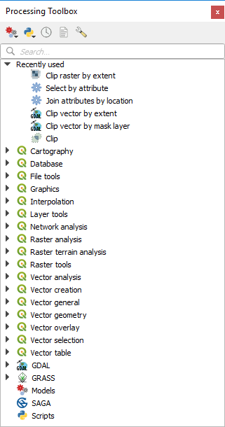
Providers can be (de)activated in the Processing settings dialog . By default, only providers that do not rely on third-party applications (that is, those that only require QGIS elements to be run) are active. Algorithms requiring external applications might need additional configuration. Configuring providers is explained in a later chapter in this manual.

In the upper part of the toolbox dialog, you will find a set of tools to:

• work with Models : Create New Model… , Open Existing Model… and Add Model to Toolbox… ;
• work with Scripts : Create New Script… , Create New Script from Template… , Open Existing Script… and Add Script to Toolbox… ;
• open the History panel;
• open the Results Viewer panel;
• toggle the toolbox to the in-place modification mode using the Edit Features In-Place button: only the algorithms that are suitable to be executed on the active layer without outputting a new layer are displayed;
• open the Options dialog.

Below this toolbar is a Search… box to help you easily find the tools you need. You can enter any word or phrase on the text box. Notice that, as you type, the number of algorithms, models or scripts in the toolbox is reduced to just those that contain the text you have entered in their names or keywords.

At the top of the list of algorithms are displayed the most recent used tools; handy if you want to reexecute any.

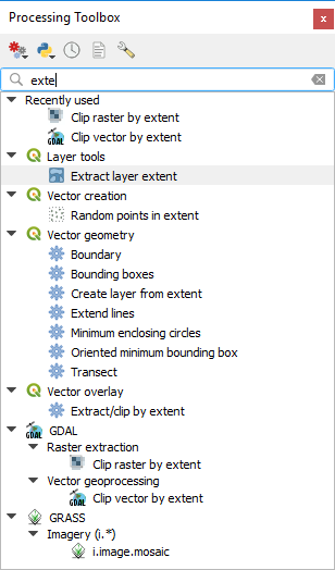
Processing Toolbox showing search results ¶

To execute a tool, just double-click on its name in the toolbox.

The algorithm dialog¶

Once you double-click on the name of the algorithm that you want to execute, a dialog similar to that in the figure below is shown (in this case, the dialog corresponds to the Centroids algorithm).

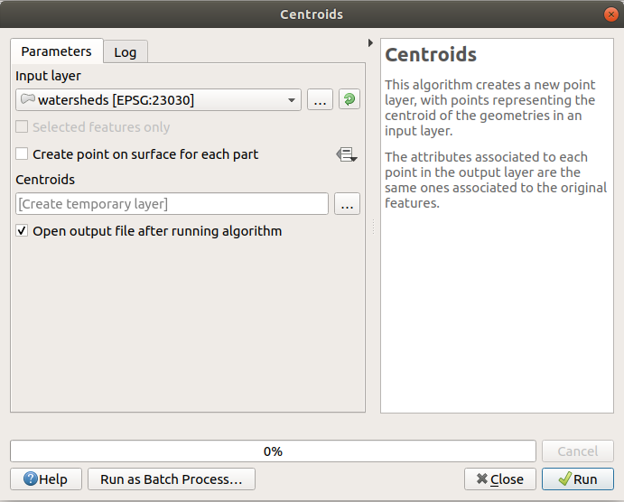
Algorithm Dialog — Parameters ¶

This dialog is used to set the input values that the algorithm needs to be executed. It shows a list of input values and configuration parameters to be set. It of course has a different content, depending on the requirements of the algorithm to be executed, and is created automatically based on those requirements.

Although the number and type of parameters depend on the characteristics of the algorithm, the structure is similar for all of them. The parameters found in the table can be of one of the following types.

• A raster layer, to select from a list of all such layers available (currently opened) in QGIS. The selector contains as well a button on its right-hand side, to let you select filenames that represent layers currently not loaded in QGIS.
• A vector layer, to select from a list of all vector layers available in QGIS. Layers not loaded in QGIS can be selected as well, as in the case of raster layers, but only if the algorithm does not require a table field selected from the attributes table of the layer. In that case, only opened layers can be selected, since they need to be open so as to retrieve the list of field names available. You will see an iterator button by each vector layer selector, as shown in the figure below.

Vector iterator button ¶

By default, the parameters dialog will show a description of the CRS of each layer along with its name. If you do not want to see this additional information, you can disable this functionality in the Processing Settings dialog, unchecking the General ‣ Show layer CRS definition in selection boxes option.

• A table, to select from a list of all available in QGIS. Non-spatial tables are loaded into QGIS like vector layers, and in fact they are treated as such by the program. Currently, the list of available tables that you will see when executing an algorithm that needs one of them is restricted to tables coming from files in dBase ( .dbf ) or Comma-Separated Values ( .csv ) formats.
• An option, to choose from a selection list of possible options.
• A numerical value, to be introduced in a spin box. In some contexts (when the parameter applies at the feature level and not at the layer’s), you will find a Data-defined override button by its side, allowing you to open the expression builder and enter a mathematical expression to generate variable values for the parameter. Some useful variables related to data loaded into QGIS can be added to your expression, so you can select a value derived from any of these variables, such as the cell size of a layer or the northernmost coordinate of another one.

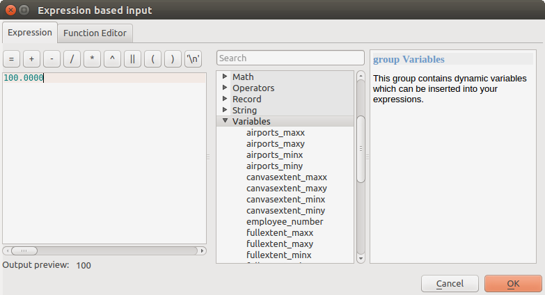
Expression based input ¶

• A range, with min and max values to be introduced in two text boxes.
• A text string, to be introduced in a text box.
• A field, to choose from the attributes table of a vector layer or a single table selected in another parameter.
• A coordinate reference system. You can select it among the recently used ones from the drop-down list or from the CRS selection dialog that appears when you click on the button on the right-hand side.
• An extent, to be entered by four numbers representing its xmin , xmax , ymin , ymax limits. Clicking on the button on the right-hand side of the value selector, a pop-up menu will appear, giving you options:
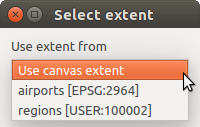
  • to select the value from a layer or the current canvas extent;
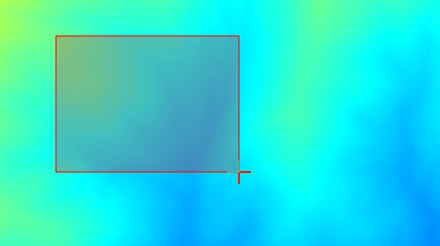
  • or to define it by dragging directly onto the map canvas.

  

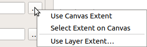
  If you select the first option, you will see a window like the next one.

  

  If you select the second one, the parameters window will hide itself, so you can click and drag onto the canvas. Once you have defined the selected rectangle, the dialog will reappear, containing the values in the extent text box.

  

  

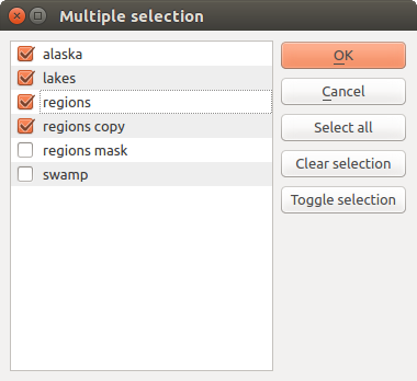
  Multiple Selection ¶

  

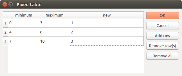
  Fixed Table ¶

  Some algorithms require many parameter to run, e.g. in the Raster calculator you have to specify manually the cell size, the extent and the CRS. You can avoid to choose all the parameters manually when the algorithm has the Reference layers parameter. With this parameter you can choose the reference layer and all its properties (cell size, extent, CRS) will be used.

  Along with the Parameters tab, there is another tab named Log (see figure below). Information provided by the algorithm during its execution is written in this tab, and allow you to track the execution and be aware and have more details about the algorithm as it runs. Notice that not all algorithms write information to this tab, and many of them might run silently without producing any output other than the final files.

  

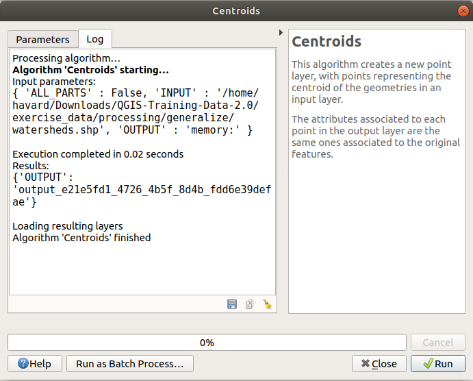
  Algorithm Dialog — Log ¶

  At the bottom of the Log tab you will find buttons to Save Log to File , Copy Log to Clipboard and Clear Log . These are particularly handy when you have checked the Keep dialog open after running algorithm in the General part of the Processing options.

  On the right hand side of the dialog you will find a short description of the algorithm, which will help you understand its purpose and its basic ideas. If such a description is not available, the description panel will not be shown.

  For a more detailed help file, which might include description of every parameter it uses, or examples, you will find a Help button at the bottom of the dialog bringing you to the Processing algorithms documentation or to the provider documentation (for some third-party providers).

  A note on projections¶

  Processing algorithm execution are always performed in the input layer coordinate reference system (CRS). Due to QGIS’s on-the-fly reprojecting capabilities, although two layers might seem to overlap and match, that might not be true if their original coordinates are used without reprojecting them onto a common coordinate system. Whenever you use more than one layer as input to a QGIS native algorithm , whether vector or raster, the layers will all be reprojected to match the coordinate reference system of the first input layer.

  This is however less true for most of the external applications whose algorithms are exposed through the processing framework as they assume that all of the layers are already in a common coordinate system and ready to be analyzed.

  By default, the parameters dialog will show a description of the CRS of each layer along with its name, making it easy to select layers that share the same CRS to be used as input layers. If you do not want to see this additional information, you can disable this functionality in the Processing settings dialog, unchecking the Show layer CRS definition in selection boxes option.

  If you try to execute an algorithm using as input two or more layers with unmatching CRSs, a warning dialog will be shown. This occurs thanks to the Warn before executing if layer CRS’s do not match option.

  You still can execute the algorithm, but be aware that in most cases that will produce wrong results, such as empty layers due to input layers not overlapping.

  Use Processing algorithms to do intermediate reprojection

  When an algorithm can not successfully perform on multiple input layers due to unmatching CRSs, use QGIS internal algorithm such as Reproject layer to perform layers’ reprojection to the same CRS before executing the algorithm using these outputs.

  Data objects generated by algorithms¶

  Data objects generated by an algorithm can be of any of the following types:

  • A raster layer
  • A vector layer
  • A table
  • An HTML file (used for text and graphical outputs)

  These are all saved to disk, and the parameters table will contain a text box corresponding to each one of these outputs, where you can type the output channel to use for saving it. An output channel contains the information needed to save the resulting object somewhere. In the most usual case, you will save it to a file, but in the case of vector layers, and when they are generated by native algorithms (algorithms not using external applications) you can also save to a PostGIS, GeoPackage or SpatiaLite database, or a memory layer.

  To select an output channel, just click on the button on the right side of the text box, and you will see a small context menu with the available options.

  In the most usual case, you will select saving to a file. If you select that option, you will be prompted with a save file dialog, where you can select the desired file path. Supported file extensions are shown in the file format selector of the dialog, depending on the kind of output and the algorithm.

  The format of the output is defined by the filename extension. The supported formats depend on what is supported by the algorithm itself. To select a format, just select the corresponding file extension (or add it, if you are directly typing the file path instead). If the extension of the file path you entered does not match any of the supported formats, a default extension will be appended to the file path, and the file format corresponding to that extension will be used to save the layer or table. Default extensions are .dbf for tables, .tif for raster layers and .gpkg for vector layers. These can be modified in the setting dialog, selecting any other of the formats supported by QGIS.

  If you do not enter any filename in the output text box (or select the corresponding option in the context menu), the result will be saved as a temporary file in the corresponding default file format, and it will be deleted once you exit QGIS (take care with that, in case you save your project and it contains temporary layers).

  You can set a default folder for output data objects. Go to the settings dialog (you can open it from the Settings ‣ Options ‣ Processing menu), and in the General group, you will find a parameter named Output folder . This output folder is used as the default path in case you type just a filename with no path (i.e., myfile.shp ) when executing an algorithm.

  When running an algorithm that uses a vector layer in iterative mode, the entered file path is used as the base path for all generated files, which are named using the base name and appending a number representing the index of the iteration. The file extension (and format) is used for all such generated files.

  Apart from raster layers and tables, algorithms also generate graphics and text as HTML files. These results are shown at the end of the algorithm execution in a new dialog. This dialog will keep the results produced by any algorithm during the current session, and can be shown at any time by selecting Processing ‣ Results Viewer from the QGIS main menu.

  Some external applications might have files (with no particular extension restrictions) as output, but they do not belong to any of the categories above. Those output files will not be processed by QGIS (opened or included into the current QGIS project), since most of the time they correspond to file formats or elements not supported by QGIS. This is, for instance, the case with LAS files used for LiDAR data. The files get created, but you won’t see anything new in your QGIS working session.

  For all the other types of output, you will find a checkbox that you can use to tell the algorithm whether to load the file once it is generated by the algorithm or not. By default, all files are opened.

  Optional outputs are not supported. That is, all outputs are created. However, you can uncheck the corresponding checkbox if you are not interested in a given output, which essentially makes it behave like an optional output (in other words, the layer is created anyway, but if you leave the text box empty, it will be saved to a temporary file and deleted once you exit QGIS).

  © Copyright 2002-now, QGIS project Last updated on Jun 05, 2020 16:39.

  7.1. Занятие: Работа с растровыми данными

  Растровые данные существенно отличаются от векторных данных. Векторные данные имеют дискретные характеристики с геометрией, которые построены из вершин и, скорее всего, связаны с линиями и/или местностями. Тем не менее растровые данные похожи на любое изображение. Хотя они могут отображать различные свойства объектов в реальном мире, эти объекты не существуют как отдельные объекты, а представлены с помощью пикселей с разными значениями.

  В этом модуле вы будете использовать растровые данные как дополнение к существующему анализу GIS.

  Цель этого урока: Научиться работать с растровыми данными в QGIS.

  7.1.1. Идем дальше: Загружаем растровые данные

  Растровые данные можно загрузить, используя те же методы, которые мы использовали для векторных данных. Тем не менее предлагается использовать панель Browser .

  1. Откройте панель Browser и расширьте папку exercise_data/raster .
  2. Загрузите все данные в эту папку:
     • 3320C_2010_314_RGB_LATLNG.tif
     • 3320D_2010_315_RGB_LATLNG.tif
     • 3420B_2010_328_RGB_LATLNG.tif
     • 3420C_2010_327_RGB_LATLNG.tif

  Вы увидите следующую карту:

  

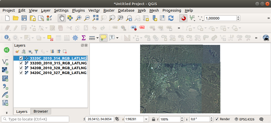
  Вот и все — четыре аэрофотоснимка местности, которую мы будем изучать.

  7.1.2. Идем дальше: Создаем виртуальный растр

  Как вы видите теперь, ваш слой расположился на всех четырех изображениях. Значит вам все время придется работать с четырьмя растрами. Это конечно не идеальный вариант. Было бы хорошо работать лишь с одним файлом.

  К счастью, QGIS дает вам возможность сделать именно это, без необходимости создавать новый растровый файл. Вы можете создать виртуальный растр, который также часто называют каталогом, что и объясняет его функцию. Это не совсем новый растр, а способ организации ваших существующих растров в одном каталоге: один файл для облегчения доступа.

  Для создания каталога мы использует Processing ► Toolbox .

  1. Откройте алгоритм Build virtual raster из GDAL ► Raster miscellaneous ;
  2. В появившемся диалоговом окне кликните на кнопку … рядом с параметром Input layers и проверьте все слои или используйте кнопку Select All ;
  3. Снимите флажок с Place each input file into a separate band . Обратите внимание на текстовое поле ниже. Это диалоговое окно на самом деле пишет этот текст за вас. Это длинная команда, которую QGIS собирается запустить.

  Примечание Помните, что вы сможете скопировать и вставить текст в OSGeo Shell (пользователь Windows) или Terminal (пользователь Linux и OSX) для того, чтобы запустить команду. Вы также можете создать запрос для каждой команды GDAL. Это очень удобно в тех случаях, когда процедура занимает много времени или когда вы хотите запланировать определенные задачи. Используйте кнопку Help для того, чтобы получить дополнительную справку по синтаксису команды.

  Как известно из предыдущих модулей, Processing создает временные слои по умолчанию. Чтобы сохранить файл, кликните на кнопку … .

  

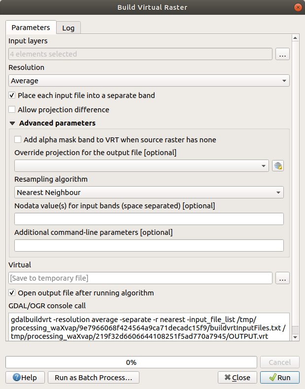
  Теперь вы можете убрать четыре исходных растра из панели Layers и оставить только выходной растр виртуального каталога.

  7.1.3. Преобразование растровых данных

  Методы, упомянутые в выше, позволят виртуально объединять наборы данных с помощью каталога и пере-проецировать их «на лету». Тем не менее, если вы настраиваете данные, которые собираетесь использовать надолго, вам лучше создать новые растры, которые уже объединены и пере-проецированы, но для первоначальной настройки может потребоваться некоторое время.

  Пере-проецирование растров

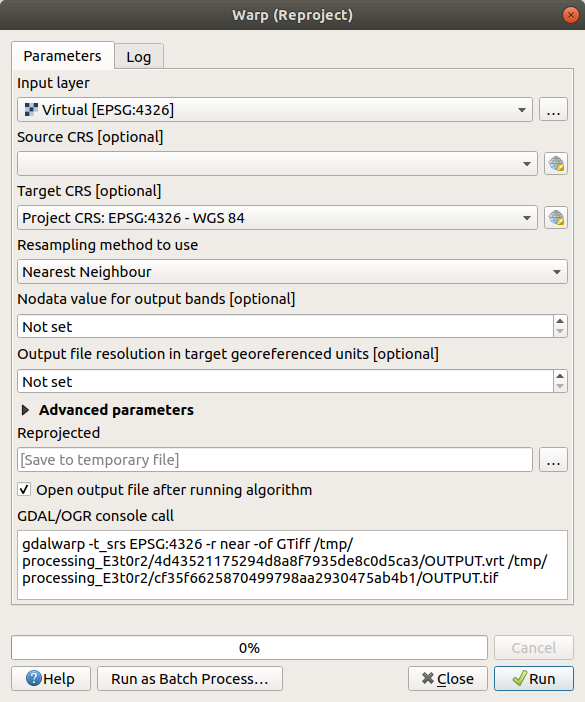
  Надо открыть Warp (reproject) в GDAL ► Raster projections .

  Вы также можете пере-проецировать виртуальные растры (каталоги), активировать многопоточную обработку и многое другое.

  

  Объединение растров

  Если вам надо создать новый растровый слой и сохранить его на диске, вы можете использовать алгоритм слияния.

  В зависимости от того, сколько растровых файлов вы объединяете и какие у них разрешения, новый растровый файл, который вы создадите, может быть довольно большого размера. Вам лучше вместо этого создать каталог растра, как описано в разделе Создать виртуальный растр .

  

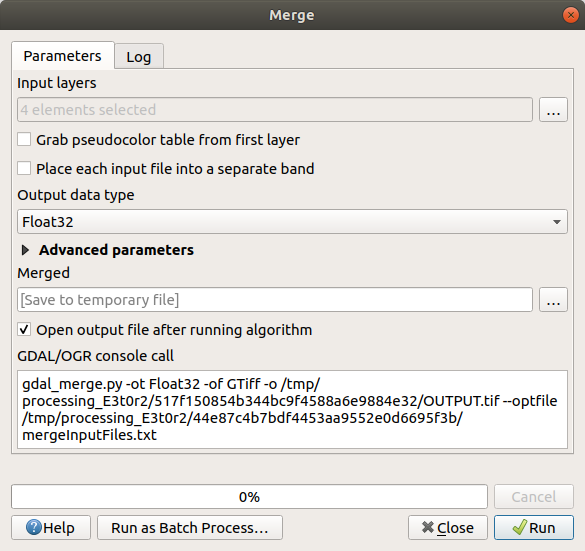
  1. Вам надо кликнуть на алгоритм СлитьОбъединить Merge в меню GDAL ► Raster miscellaneous .
  2. Как и в случае с Созданием виртуального растра , используйте кнопку … для того, чтобы выбрать, какие слои вы хотите объединить. Вы также можете указать виртуальный растр в качестве входных данных, и тогда все растры, из которых он состоит, будут обработаны.
  3. Если вы знаете библиотеку GDAL, вы также можете добавить свои собственные опции, открыв меню Advanced parameters .

  7.1.4. В заключении

  QGIS облегчает включение растровых данных в ваши существующие проекты.

  7.1.5. Что дальше?

  Далее мы собираемся использовать растровые данные, которые не являются аэрофотоснимками, чтобы увидеть, как символы могут быть полезными и в случае с растрами.

  © Copyright 2002-now, QGIS project. Обновлено: апр. 02, 2022 16:05.

  Читать:

  Как вернуть в иллюстраторе способ растягивания картинки