Как получить функцию от ndsolve в mathematica

Numerical Solution of Partial Differential Equations

The Wolfram Language function NDSolve has extensive capability for solving partial differential equations (PDEs). A unique feature of NDSolve is that given PDEs and the solution domain in symbolic form, NDSolve automatically chooses numerical methods that appear best suited to the problem structure. Commonly, the automatic algorithm selection works quite well, but it is useful to have an understanding of the methods used, both to better understand the solutions provided and to use method options to get better solutions or improve efficiency.

NDSolve [ < eqn ₁ , eqn ₂ , … > , u , < x , x _min , x _max > , < y , y _min , y _max > ]	find a numerical solution of < eqn ₁ , eqn ₂ , … > for the function u [ x , y ] over the rectangular domain [ x _min , x _max ] × [ y _min , y _max ]
NDSolve [ < eqn ₁ , eqn ₂ , … > , u , < x , y >∈ Ω ]	find a numerical solution of < eqn ₁ , eqn ₂ , … > for the function u [ x , y ] over the domain Ω
NDSolve [ < eqn ₁ , eqn ₂ , … > , u , < t , t _min , t _max > , < x , y >∈ Ω ]	find a numerical solution of the time-dependent equations < eqn ₁ , eqn ₂ , … > for the function u [ t , x , y ] over the spatial domain Ω for times between t _min and t _max .

Finding numerical solutions to partial differential equations with NDSolve . NDSolve uses finite element and finite difference methods for discretizing and solving PDEs. The numerical method of lines is used for time-dependent equations with either finite element or finite difference spatial discretizations, and details of this are described in the tutorial «The Numerical Method of Lines». Finite element methods are more general and are described extensively in their own tutorials. The following examples give a brief introduction to how equations may be entered and methods are automatically chosen.

Load a package useful for examining solutions:
Solve a Poisson equation in two variables on a rectangular region with zero boundary conditions:

The input above uses notation with derivatives given explicitly. For some problems it is more expressive and correct to use an operator form. By default, the common operators Grad , Div , Curl , and Laplacian evaluate automatically, but for expressing PDEs it is typically better not to have these evaluate. It is possible to maintain the operator form using Inactive . In general, Inactive [ f ] represents an inactive form of f that does not evaluate. Inactive forms can be activated using Activate , but commands like NDSolve can also work with the inactive forms directly.

Evaluated and Inactive form of a differential operator:

Note that the inactive form has retained meaning from the operator form that might be lost with the explicit evaluation; for example, if were discontinuous, the derivative expressions would be indeterminate, whereas the operator expression can be well defined if has discontinuities corresponding to those of . A convenient way to get inactive operators is to use Inactivate with the operators you want inactivated given in the pattern in the second argument.

Perhaps the most convenient and certainly the most readable way to enter equations is to just use the typeset forms. These can be obtained by copying and pasting the output of inactive forms or by using the escape sequences given in the reference pages for each of the operators.

Typeset form for the Laplacian:

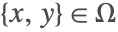
In the example above, the zero boundary conditions were given as explicit equations. An alternative is to use DirichletCondition [ eqn , pred ] , which specifies that eqn should be satisfied everywhere on the boundary of the domain where pred is True . Generalized Neumann boundary conditions may be specified using NeumannValue ; since this is specific to the finite element method, the description of NeumannValue will be found in the finite element method tutorials. Typically, the spatial variables are restricted to some domain, and NDSolve recognizes the notation .

Solving a nicely typeset form of the Poisson equation:

This solution is the same as the one shown above, and both are computed using the finite element method. The automatic selection was done this for this example because both and have boundary conditions; the method of lines requires that there be an initial value problem for one of the independent variables. The finite element method uses a mesh to compute the solution. You can see the mesh by extracting it from the solution.

Get the mesh from the solution and show its wire frame:

The finite element method is good at handling nonrectangular geometries as well. All that needs to be done to solve the problem over a different domain is to define that domain.

Solve the Poisson equation over the unit disk:

Some of the visualization commands accept the domain notation, so you can use them directly for visualizing the solution.

Show the solution:
Show the mesh used to find the solution:
In some cases it is possible to see the mesh with a plot by using the option Mesh->All .
Show the plot of the solution surface along with the mesh:

NDSolve handles equations that have an independent variable that is time-like, in the sense that the solution evolves so that variables from specified initial conditions are solved using the numerical method of lines with either a finite difference or finite element spatial discretization. Consider as an example the problem of finding out how long it takes to get the center of a plate to a prescribed temperature from when steady heat is applied to the outside. This is modeled by the heat equation.

Solve the plate-heating problem for a rectangular plate:
Plot the solution at the final time:

When the region is rectangular, NDSolve uses finite differences by default; it is possible to specify the type and even specific details for the spatial discretization using Method options. The tutorials about method of lines and finite element methods give detailed information about the options and many examples using them.

Introduction to Advanced Numerical Differential Equation Solving in the Wolfram Language

The Wolfram Language function NDSolve is a general numerical differential equation solver. It can handle a wide range of ordinary differential equations (ODEs) as well as some partial differential equations (PDEs). In a system of ordinary differential equations there can be any number of unknown functions u _i , but all of these functions must depend on a single «independent variable» t , which is the same for each function. Partial differential equations involve two or more independent variables. NDSolve can also solve some differential-algebraic equations (DAEs), which are typically a mix of differential and algebraic equations.

NDSolve [ < eqn ₁ , eqn ₂ , … > , u , < t , t _min , t _max > ]	find a numerical solution for the function u with t in the range t _min to t _max
NDSolve [ < eqn ₁ , eqn ₂ , … > , < u ₁ , u ₂ , … > , < t , t _min , t _max > ]	find numerical solutions for several functions u _i

Finding numerical solutions to ordinary differential equations. NDSolve represents solutions for the functions u _i as InterpolatingFunction objects. The InterpolatingFunction objects provide approximations to the u _i over the range of values t _min to t _max for the independent variable t . In general, NDSolve finds solutions iteratively. It starts at a particular value of t , then takes a sequence of steps, trying eventually to cover the whole range t _min to t _max . In order to get started, NDSolve has to be given appropriate initial or boundary conditions for the u _i and their derivatives. These conditions specify values for u _i [ t ] , and perhaps derivatives u _i ‘ [ t ] , at particular points t . When there is only one t at which conditions are given, the equations and initial conditions are collectively referred to as an initial value problem. A boundary value occurs when there are multiple points t . NDSolve can solve nearly all initial value problems that can symbolically be put in normal form (i.e. are solvable for the highest derivative order), but only linear boundary value problems.

This finds a solution for x with t in the range 0 to 2, using an initial condition for x at t  1 :

When you use NDSolve , the initial or boundary conditions you give must be sufficient to determine the solutions for the u _i completely. When you use DSolve to find symbolic solutions to differential equations, you may specify fewer conditions. The reason is that DSolve automatically inserts arbitrary symbolic constants C [ i ] to represent degrees of freedom associated with initial conditions that you have not specified explicitly. Since NDSolve must give a numerical solution, it cannot represent these kinds of additional degrees of freedom. As a result, you must explicitly give all the initial or boundary conditions that are needed to determine the solution. In a typical case, if you have differential equations with up to th derivatives, then you need to either give initial conditions for up to th derivatives, or give boundary conditions at points.

This solves an initial value problem for a second-order equation, which requires two conditions, given at t  0 :

Preface

This section is about application of standard Mathematica command NDSolve to the systems of ordinary differential equations.

Contents [hide]

Preface
1. Introduction
  1. 3D plotting
  2. Tubing
  3. Existence and Uniqueness
  4. Picard iterations
  5. Adomian iterations
  6. Euler—Lagrange equations
  7. Lagrange multipliers
  8. Hamilton principle
  9. Converting to a system
2. Part I:Matrix Algebra
  1. How to define vectors
  2. How to define matrices
  3. Basic operations with matrices
  4. Linear systems of equations
  5. Determinants and inverses
  6. Special matrices
  7. Eigenvalues and Eigenvectors
  8. Diagonalization procedure
  9. Sylvester formula
  10. The resolvent method
  11. Polynomial interpolation
  12. Positive matrices
  13. Roots
  14. Miscellany
3. Part II:Linear Systems of Ordinary Differential Equations
  1. Variable coefficient systems of ODEs
  2. Constant coefficient systems of ODEs
  3. Planar Phase Portrait
  4. Euler systems of equations
  5. Fundamental matrices
  6. Reduction to a single equation
  7. Method of undetermined coefficients
  8. Variation of parameters
  9. Laplace transform
  10. Second order ODEs
  11. Spring-mass systems
  12. Electric circuits
  13. Applications
4. Part III:Non-linear Systems of Ordinary Differential Equations
  1. Planar autonomous systems
  2. Numerical solutions
  3. Stability
  4. Linearization
  5. Pendulum
    1. Phase Portrait
    2. Moving pivot
    3. Numerical simulation
    4. Sprung pendulum
    5. Elastic pendulum
    6. Double pendulum
    7. Escapement
    8. Inverted pendulum
    9. ADM approximation
    10. Fourier series
  6. Spring-mass system
    1. Anharmonic motion
    2. Forced anharmonic motion
    3. Duffing equations
    4. Forced Duffing equation
    5. Driven hard spring
    6. Driven soft spring
    7. Coulomb damping
    8. Quadratic damping
  7. Conservative systems
  8. Gradient systems
  9. Competing species
  10. Predator-Prey equations
  11. Harvesting species
  12. Lyapunov second method
  13. Periodic solutions
  14. Asynchronous solutions
  15. Limited Cycles
  16. van der Pol equations
  17. Chaos
  18. Lorenz equations
  19. Rössler attractor
  20. Neuroscience
  21. Electric circuits
  22. Chua circuits
  23. Mechanical problems
  24. Miscellany
5. Part IV:Numerical Methods
  1. Iterative methods
  2. Iterations for nonlinear systems
  3. Numerical solutions using NDSolve
  4. Euler’s methods
  5. Runge—Kutta methods
  6. Finite Difference Methods
  7. Adomian Decomposition Method
  8. Variational iteration method
  9. Finite Element Method
  10. Second order ODEs
  11. Applications
6. Part V:Fourier Series
  1. Sturm—Liouville problems
  2. Fourier transform
  3. Fourier series
  4. Periodic extension
  5. Complex Fourier series
  6. Even and odd functions
  7. Examples
  8. Gibbs phenomenon
  9. Convergence of Fourier series
  10. Cesàro summation
  11. Square wave functions
  12. Orthogonal expansions
  13. Chebyshev expansions
  14. Legendre expansion
  15. Bessel expansion
  16. Hermite expansion
  17. Laguerre expansion
  18. Motivated examples
7. Part VI:Partial Differential Equations
  1. First order PDEs
  2. Separation of variables
  3. Parabolic equations
    1. Heat conduction problems
    2. Boundary Value Problems for heat equation
    3. Other heat transfer problems
    4. Fourier transform
    5. Numerical solutions of heat equation
    6. Black Scholes model
    7. Monter Carlo for Parabolic
  4. Hyperbolic equations
    1. Wave equations
    2. 2D wave equations
    3. Forced wave equations
    4. Transverse vibrations of beams
    5. Numerical solutions of wave equation
  5. Elliptic equations
    1. Laplace equation
    2. Dirichlet problem
    3. Neumann problems for Laplace equation
    4. Mixed problems for Laplace equation
    5. Laplace equation in infinite stripe
    6. Laplace equation in infinite semi-stripe
    7. Numerical solutions of Laplace equation
    8. Laplace equation in polar coordinates
    9. Laplace equation in a corner
    10. Laplace equation in spherical coordinates
    11. Poisson’s equation
    12. Helmholtz equation
    13. Liouville’s equation
    14. Monter Carlo for Elliptic
  6. Green’s functions
  7. Blasius equation
  8. Applications
  9. Miscellany
8. Part VII:Special Functions
  1. Orthogonal polynomials
  2. Gamma function
  3. Bessel functions
  4. Orthogonality of Bessel functions
  5. Airy functions
  6. Lambert function
  7. Mathieu function
  8. Chebyshev functions
  9. Legendre functions
  10. Elliptic functions
  11. Hypergeometric functions
  12. Miscellany

Читать:

Как скачать мод на бесконечное лето на ios

Return to computing page for the first course APMA0330
Return to computing page for the second course APMA0340
Return to Mathematica tutorial for the first course APMA0330
Return to Mathematica tutorial for the second course APMA0340
Return to the main page for the first course APMA0330
Return to the main page for the second course APMA0340
Return to Part IV of the course APMA0340
Introduction to Linear Algebra with Mathematica

Glossary

Numerical solutions using NDSolve

The Wolfram Language function NDSolve is a general numerical differential equation solver. It can handle a wide range of ordinary differential equations (ODEs) as well as some partial differential equations (PDEs) and some differential-algebraic equations (DAEs). In a system of ordinary differential equations, there can be any number of unknown functions, but all of these functions must depend on a single independent variable, which is the same for each function. NDSolve provides approximations to the solutions as InterpolatingFunction objects over the specified range of independent variable.

In order to get started, NDSolve has to be given appropriate initial or boundary conditions for the which the problem has a unique solution. These conditions specify values for the unknown function/solution, and perhaps its derivatives, if needed. A boundary value occurs when the unknown function is specified at multiple points. NDSolve can solve nearly all initial value problems that can symbolically be put in normal form (i.e. are solvable for the highest derivative order), but only linear boundary value problems. Example: forced pendulum equation

Example: Consider the driven pendulum that is modeled by the following initial value problem:

\[ \ddot (t) + \sin \left( x (t) \right) = 4\,\sin (2t) , \qquad x(0) =1, \quad \dot (0) =0. \]

This pendulum is set into motion with no initial velocity, denoted by \( \dot , \) and it is subject by the periodic external force, 4 sin(2t). As usual, we denote the independent variable by t associated with time, and denote derivatives of x (which is angle of inclination with respect to downward position of a bob of unit mass) by dots. Here is the code to determine the approximate solution in the interval t ∈ [0, 100].

solution = NDSolve[, x, ]
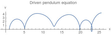
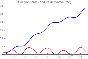
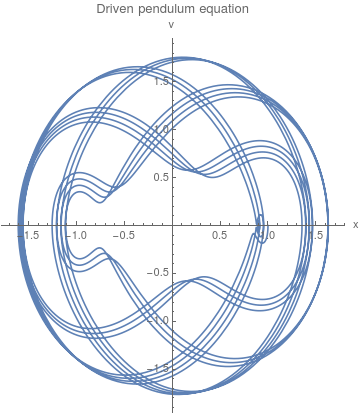
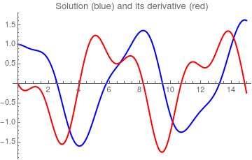
\( \left\< \left\< x \to \mbox\left[ \begin \mbox\\> \\ \mbox \end \right] \right\> \right\> \)

Next we plot separately the solution and its derivative/velocity and the using ParametricPlot we plot x vs its derivative, denoted by v.

Plot[Evaluate[ /. solution], , PlotRange -> All, PlotStyle -> , >, PlotLabel -> «Solution (blue) and its derivative (red)» ]
ParametricPlot[ /. solution, , AxesLabel -> , PlotLabel -> «Driven pendulum equation»]

■

As mentioned earlier, NDSolve works by taking a sequence of steps in the independent variable t. NDSolve uses an adaptive procedure to determine the size of these steps. In general, if the solution appears to be varying rapidly in a particular region, then NDSolve will reduce the step size to be able to better track the solution. NDSolve allows you to specify the precision or accuracy of result you want. In general, NDSolve makes the steps it takes smaller and smaller until the solution reached satisfies either the AccuracyGoal or the PrecisionGoal you give. The setting for AccuracyGoal effectively determines the absolute error to allow in the solution, while the setting for PrecisionGoal determines the relative error. If you need to track a solution whose value comes close to zero, then you will typically need to increase the setting for AccuracyGoal. By setting AccuracyGoal->Infinity, you tell NDSolve to use PrecisionGoal only. Generally, AccuracyGoal and PrecisionGoal are used to control the error local to a particular time step. For some differential equations, this error can accumulate, so it is possible that the precision or accuracy of the result at the end of the time interval may be much less than what you might expect from the settings of AccuracyGoal and PrecisionGoal .

NDSolve uses the setting you give for WorkingPrecision to determine the precision to use in its internal computations. If you specify large values for AccuracyGoal or PrecisionGoal , then you typically need to give a somewhat larger value for WorkingPrecision. With the default setting of Automatic, both AccuracyGoal and PrecisionGoal are equal to half of the setting for WorkingPrecision . NDSolve uses the setting you give for WorkingPrecision to determine the precision to use in its internal computations.

NDSolve follows the general procedure of reducing step size until it tracks solutions accurately. There is a problem, however, when the true solution has a singularity. In this case, NDSolve might go on reducing the step size forever, and never terminate. To avoid this problem, the option MaxSteps specifies the maximum number of steps that NDSolve will ever take in attempting to find a solution. For ordinary differential equations, the default setting is MaxSteps->10000. The default setting MaxSteps->10000 should be sufficient for most equations with smooth solutions. When solutions have a complicated structure, however, you may sometimes have to choose larger settings for MaxSteps . With the setting MaxSteps->Infinity there is no upper limit on the number of steps used. Example: driven pendulum and Duffing equations

Example: The pendulum equation contains sine function depending on the angle of inclination. If we approximate this sine function by its two term Maclaurin series \( \sin x \approx x — \frac + \cdots , \) we come to the so called the Duffing equation (undamped):

\[ \ddot (t) + y — \frac = 4\,\sin (2t) , \qquad y(0) =1, \quad \dot (0) =0. \]

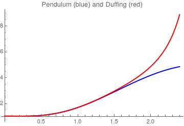
We expect that the solutions to the corresponding initial value problem of the above Duffing equation will be closed to our pendulum equation. However, it is not the case, as the following graphs show.

duffing = NDSolve[, y, ]

. NDSolve: At t == 2.8049247505261308`, step size is effectively zero; singularity or stiff system suspected.

So we use WorkingPrecision option:
duf100 = NDSolve[, y, , WorkingPrecision -> 30]

. NDSolve: At t == 2.8049248718686542658960305575797542678549496716458439572537`30., step size is effectively zero; singularity or stiff system suspected.

When we plot two solutions, for the pendulum equation and for Duffing equations, we see that the coincide only within short time interval

Plot[Evaluate[ ], , PlotRange -> All, PlotStyle -> , >, PlotLabel -> «Pendulum (blue) and Duffing (red)» ]

When we increase the interval, we come to a similar problem:

sol150 = NDSolve[, x, , WorkingPrecision -> 30]

. NDSolve: Maximum number of 10000 steps reached at the point t == 102.17448133270418317650562000181362967153`30..

This message actually indicates that the solution of this driven pendulum equation is unbounded. We try to reduce the amplitude of the oscillating force:

sol150 = NDSolve[, x, , WorkingPrecision -> 30]
ParametricPlot[ /. sol150, , AxesLabel -> , PlotLabel -> «Driven pendulum equation»]
Plot[Evaluate[ /. sol150], , PlotRange -> All, PlotStyle -> , >, PlotLabel -> «Solution (blue) and its derivative (red)» ]

Then we repeat calculations with the same driven force for Duffing equation.
You can also specify the solution method:
duf150 = NDSolve[, y, , WorkingPrecision -> 30, Method -> «ExplicitRungeKutta»]

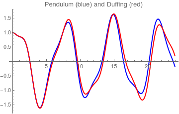
However, upon plotting, we will not recognize the difference. As we see, for such amplitude (equals 1), both equations have bounded solutions that we very closed. ■

When NDSolve computes a solution, there are typically three phases. First, the equations are processed, usually into a function that represents the right-hand side of the equations in normal form. Next, the function is used to iterate the solution from the initial conditions. Finally, data saved during the iteration procedure is processed into one or more InterpolatingFunction objects. Using functions in the NDSolve` context, you can run these steps separately and, more importantly, have more control over the iteration process. The steps are tied by an NDSolve`StateData object, which keeps all of the data necessary for solving the differential equations.

Boccio, John, Advanced Numerical Differential Equation Solving in Mathematica, 2008.
Introduction to Advanced Numerical Differential Equation Solving in the Wolfram Language.

Return to Mathematica page
Return to the main page (APMA0340)
Return to the Part 1 Matrix Algebra
Return to the Part 2 Linear Systems of Ordinary Differential Equations
Return to the Part 3 Non-linear Systems of Ordinary Differential Equations
Return to the Part 4 Numerical Methods
Return to the Part 5 Fourier Series
Return to the Part 6 Partial Differential Equations
Return to the Part 7 Special Functions