
What Is Antenna Toolbox?
Design, analyze, and visualize antenna elements and antenna arrays using Antenna Toolbox™. You can design standalone antennas and build linear and rectangular arrays of antennas using a library of predefined elements with parameterized geometry. For example, you can design Yagi, loop, patch and PIFA antennas for wireless communication and radar systems.
Antenna Toolbox uses the method of moments (MoM) to compute port properties such as impedance, surface properties such as current and charge distribution, and field properties such as the far field radiation pattern. Antenna Toolbox provides impedance analysis that can be used to design matching networks with RF Toolbox™. It also provides radiation patterns for simulating beamforming algorithms together with Phased Array System Toolbox™.
With examples, you can rapidly start designing antennas and antenna arrays and use the results for antenna-to-bits wireless system design.
installedAntenna
The installedAntenna object creates an installed antenna setup that enables you to mount antennas on a platform for analysis.
Installed antenna analysis involves an electrically large structure called a platform. Around this platform, different antenna elements are placed. You can analyze the effects of the platform on the antenna performance. Installed antenna analysis is commonly used in aerospace, defense, and auto applications. The platform in this case are plane, ship, or an automobile.
Another common application of installed antenna analysis is to determine the interference of different antennas placed on a large platform.
Note
installedAntenna only models pure metal structures.
Creation
Syntax
Description
ant = installedAntenna creates an installed antenna setup. The default setup has a rectangular reflector in the xy-plane as the platform with a dipole as the antenna. The dimensions of the dipole antenna are chosen for an operating frequency of 1GHz.
ant = installedAntenna(Name=Value) creates an installed antenna setup, with additional Properties specified by one or more name-value arguments. Name is the property name and Value is the corresponding value. You can specify several name-value pair arguments in any order as Name1=Value1 , . , NameN=ValueN . Properties that you do not specify retain their default values.
Output Arguments
ant — Installed antenna setup
installedAntenna object
Installed antenna setup, returned as an installedAntenna object.
Properties
Platform — Platform object file
platform object
Platform object file, specified as a platform object.
Example: platform(FileName=’plate.stl’)
Data Types: char
Element — Single or multiple antenna elements
antenna object | cell array of antenna objects
Single or multiple antennas, specified as an antenna object or a cell array of antenna objects. For multiple antenna elements, you must specify ElementPosition for all the elements.
Example: dipole
Example: ant = installedAntenna(Element=, ElementPosition=[0.1 0.1 0.5; -0.1 -0.1 0.5]) This code creates discone and monocone antenna objects for installed antenna analysis.
Data Types: char
ElementPosition — Position of feed or origin of each antenna element
[0 0 0.0750] (default) | vector of [x,y,z] coordinates
Position of the feed or the origin of each antenna element, specified as a vector of [x,y,z] coordinates in meters. For multiple antenna elements, the number of positions in ElementPosition must be equal to the number of elements specified in the Element property.
Example: [0 0 0.0050]
Data Types: double
Reference — Reference for positioning antenna elements
«feed» (default) | «origin»
Reference for positioning the antenna elements, specified as either «feed» or «origin» .
Example: «origin»
Data Types: string
FeedVoltage — Excitation amplitude for antenna elements
1 (default) | vector
Excitation amplitude for the antenna elements, specified as a scalar vector in volts. For multiple antenna elements, the number of elements in FeedVoltage must be equal to the number of elements specified in the Element property.
Example: 2
Example: [2 5]
Data Types: double
FeedPhase — Phase shift of each antenna element
0 (default) | vector
Phase shift of each antenna element, specified as a scalar or vector in degrees. For multiple antenna elements, the number of elements in FeedPhase must be equal to the number of elements specified in the Element property.
Example: 50
Example: [50 60]
Data Types: double
Tilt — Tilt angle of antenna
0 (default) | scalar | vector
Tilt angle of the antenna in degrees, specified as a scalar or vector. For more information, see Rotate Antennas and Arrays.
Example: 90
Example: Tilt=[90 90] , TiltAxis=[0 1 0;0 1 1] tilts the antenna at 90 degrees about the two axes defined by the vectors.
Data Types: double
TiltAxis — Tilt axis of antenna
[1 0 0] (default) | three-element vector | 2-by-3 matrix | «X» | «Y» | «Z»
Tilt axis of the antenna, specified as one of these values:
- Three-element vector of Cartesian coordinates in meters. In this case, each coordinate in the vector starts at the origin and lies along the specified points on the x-, y-, and z-axes.
- Two points in space, specified as a 2-by-3 matrix corresponding to two three-element vectors of Cartesian coordinates. In this case, the antenna rotates around the line joining the two points.
- «x» , «y» , or «z» to describe a rotation about the x-, y-, or z-axis, respectively.
Example: [0 1 0]
Example: [0 0 0;0 1 0]
Example: «Z»
Data Types: double | string
SolverType — Solver for antenna analysis
«MoM-PO» (default) | «MoM» | «FMM»
Solver for antenna analysis, specified as either «MoM-PO» (Method of Moments-Physical Optics) or «MoM» (Method of Moments) or «FMM» (Fast Multipole Method).
Example: «MoM»
Data Types: string
Object Functions
| show | Display antenna, array structures, shapes, or platform |
| axialRatio | Axial ratio of antenna |
| beamwidth | Beamwidth of antenna |
| charge | Charge distribution on antenna or array surface |
| current | Current distribution on antenna or array surface |
| efficiency | Radiation efficiency of antenna |
| EHfields | Electric and magnetic fields of antennas or embedded electric and magnetic fields of antenna element in arrays |
| impedance | Input impedance of antenna or scan impedance of array |
| mesh | Mesh properties of metal, dielectric antenna, or array structure |
| meshconfig | Change meshing mode of antenna, array, custom antenna, custom array, or custom geometry |
| pattern | Plot radiation pattern and phase of antenna or array or embedded pattern of antenna element in array |
| patternAzimuth | Azimuth plane radiation pattern of antenna or array |
| patternElevation | Elevation plane radiation pattern of antenna or array |
| rcs | Calculate and plot radar cross section (RCS) of platform, antenna, or array |
| returnLoss | Return loss of antenna or scan return loss of array |
| solver | Access FMM solver for electromagnetic analysis |
| sparameters | Calculate S-parameters for antennas and antenna arrays |
| vswr | Voltage standing wave ratio (VSWR) of antenna or array element |
Examples
Installed Antenna Setup and Analysis
Create a default installed antenna.
ant = installedAntenna
ant = installedAntenna with properties: Platform: [1x1 platform] Element: [1x1 dipole] ElementPosition: [0 0 0.0750] Reference: 'feed' FeedVoltage: 1 FeedPhase: 0 Tilt: 0 TiltAxis: [1 0 0] SolverType: 'MoM-PO'
show(ant);
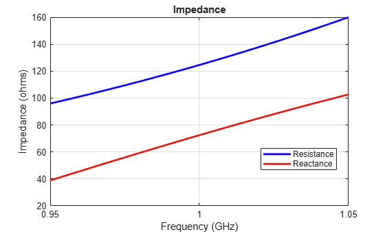
Calculate the impedance of the antenna.
figure; impedance(ant, linspace(950e6, 1050e6, 51));
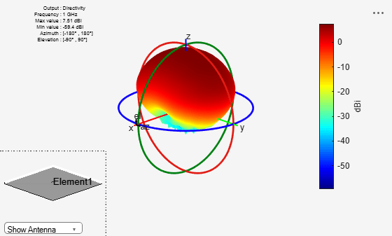
Visualize the pattern of the antenna.
figure; pattern(ant, 1e9);
Radiation Pattern of Antenna Installed on Glider
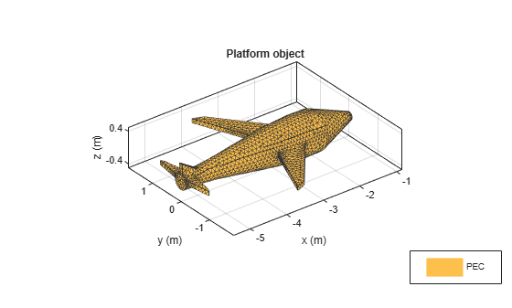
Create a platform from the STL file containing geometry infomation of a glider.
plat = platform(FileName="glider.stl", Units="m"); figure show(plat);
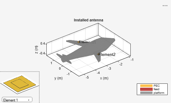
Design a dipole antenna operating at 1GHz. Install this dipole antenna element below the nose of the glider.
d = design(dipole,1e9); d.Tilt = 90; d.TiltAxis=[1 0 0]; ant = installedAntenna(Platform=plat, Element=d, ElementPosition=[-1.2 0 -0.25]); figure show(ant);
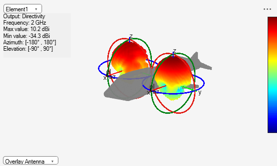
Visualize the radiation pattern of the installed dipole.
figure pattern(ant,1e9)
Algorithms
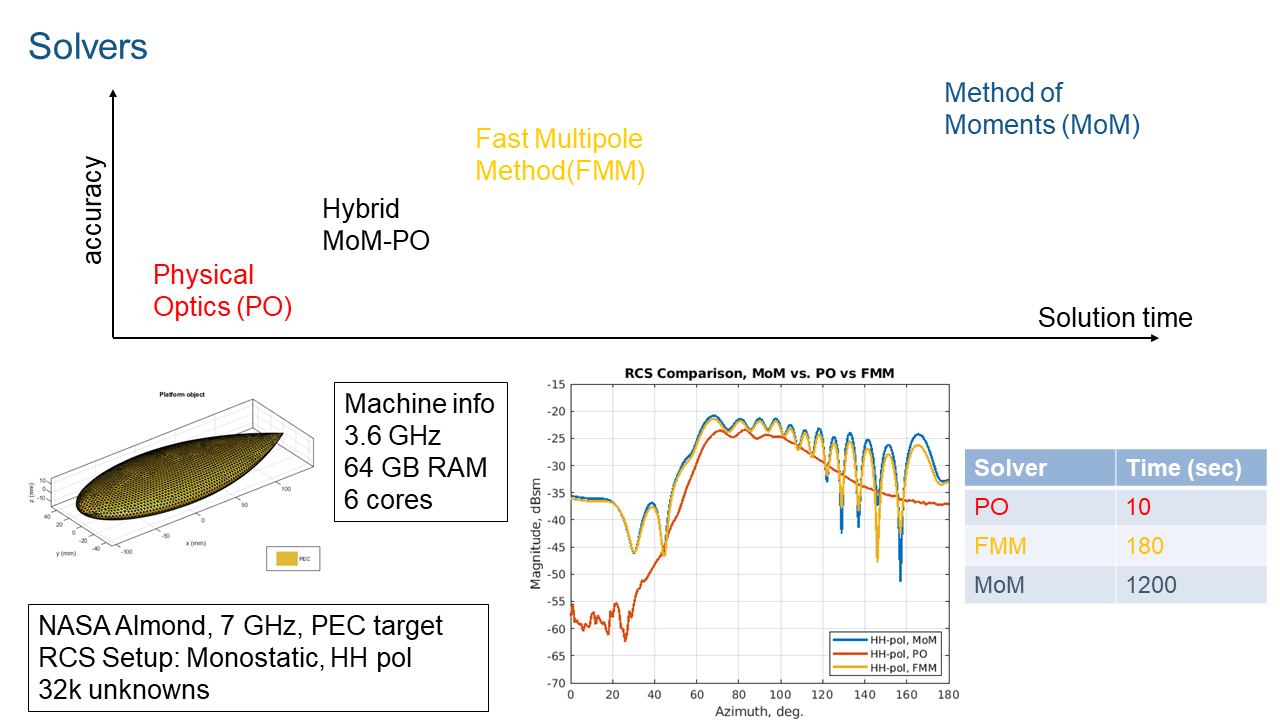
Solver Recommendations for Installed Antenna Analysis
Hybrid MoM PO Solver
The default solver for installed antenna analysis is the hybrid MoM-PO ( Method of moments and physical optics) solver. This is a hybrid solver, with less stringent requirements on the mesh. This approach does not have full-wave accuracy since the electrically large portion of the geometry is handled using the physical optics approach. For more information on this solver see, Hybrid MoM-PO Method for Metal Antennas with Large Scatterers.
FMM Solver
For full wave accuracy in installed antenna analysis you can use the FMM (fast multiple method) solver. This solver does not fill and store a matrix of interactions and enables the solution of large structures which is not possible when using the MoM solver. For open geometries, this solver builds a preconditioner matrix internally. The preconditioner matrix is sparse but might be less sparse for larger structures. Preconditioner matrices are not built for closed geometries. When using the FMM, you have an option to use the solver object to set up the number of iterations and the relative error. In some circumstances it might be useful to study the nature of the problem and its convergence characteristics by reducing the number of iterations or the relative error initially or both. The FMM solver does need approximately 10 elements per wavelength in the mesh. The number of elements does impact the convergence of the solution. For more information on FMM solvers, see Fast Multipole Method for Large Structures.
MoM Solver
For wavelength and sub-wavelength scale structures, with or without dielectric you can use an MoM (method of moments)solver. For more information on MoM solver, see Method of Moments Solver for Metal Structures and Method of Moments Solver for Metal and Dielectric Structures.
Get Started with Antenna Toolbox
Antenna Toolbox™ provides functions and apps for the design, analysis, and visualization of antenna elements and arrays. You can design standalone antennas and build arrays of antennas using predefined elements with parameterized geometry, arbitrary planar structures, or custom 3D structures described with STL files.
Antenna Toolbox uses electromagnetic solvers, including the method of moments (MoM), to compute impedance, current distribution, efficiency, and near-field and far-field radiation patterns. To improve the antenna design, you can use manual methods or use the optimization methods provided in the toolbox. Antenna geometry and analysis results can be visualized in 2D and 3D. The toolbox lets you integrate antenna array patterns into wireless systems for simulating beamforming and beam steering algorithms. The impedance analysis results can be used to design matching networks for integration with the RF front-end. You can install the antennas on large platforms such as vehicles or aircraft and analyze the effects of the structure on antenna performance. You can import STL and Gerber files to analyze a pre-existing structure or export them to share or manufacture your design. A site viewer enables you to visualize antenna coverage on a 3D terrain map using a variety of propagation models, including ray tracing.
Tutorials
Apps
- Design and Analysis Using Antenna Designer
Interactively construct, analyze and export antenna using Antenna Designer app. - Design and Analysis Using Antenna Array Designer
Interactively create and analyze antenna arrays using Antenna Array Designer app. - Design and Analysis Using PCB Antenna Designer
Design, validate, analyze, and export 1-by-2 H-notch linear antenna array.- STEP 1: Define PCB Antenna Layers
- STEP 2: Design H-Notch Patch Unit Element
- STEP 3: Analyze H-Notch Unit Element
- STEP 4: Design, Analyze, and Export 1-by-2 H-Notch Linear Array
- STEP 5: Design, Analyze, and Optimize H-Notch Patch Using Design Variables
Modelling, Analysis, and Visualization
- Antenna Modeling and Analysis
Construct, visualize and analyze antenna elements. - Array Modeling and Analysis
Construct, visualize, and analyze an antenna array. - Interact with Polar Plot
Use the interactivity features of a polar plot. - RF Propagation and Visualization
Visualize coverage maps, SINR maps, and propagation paths in outdoor and indoor environments.
More About
Fundamental Analysis of Antennas
- Port Analysis
Input impedance, resonance, return loss, reflection coefficient, bandwidth. - Surface Analysis
Charge distribution, current distribution. - Field Analysis
Radiation pattern, E-H fields, beamwidth, polarization, axial ratio. - Far-field Terminologies
Antenna gain, directivity and realized gain.
Array Analysis
- Mutual Coupling
Active or scan impedance, array factor and pattern multiplication, coupling matrix, isolated or embedded element pattern. - Correlation Coefficient
Far-field radiation pattern, S-parameter characterization. - Beamforming
Side lobe control, beam scanning. - Grating Lobes
Grating lobes are the maxima of the main beam, as predicted by the pattern multiplication theorem.
Antenna Modeling
- Antenna Classification
Classify antennas based on radiation pattern or feeding mechanism. - Antenna Toolbox Coordinate System
Rectangular and spherical coordinate system. - Antenna Radiation Patterns
Default radiation patterns of built-in antennas. - Feed Model
Antenna Toolbox feed model. - Meshing
Method of Moments (MoM) is a numerical method that transforms Maxwell’s continuous integral equations into an approximate discrete formulation that requires inversion of a large matrix. - Solvers
Different types of solvers, solver applications.
Featured Examples
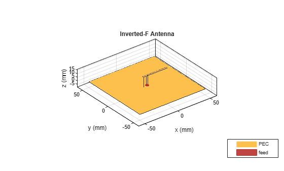
Port Analysis of Antenna
Quantifies terminal antenna parameters, with regard to the antenna port. The antenna is a one-port network. The antenna port is a physical location on the antenna where an RF source is connected to it. The terminal port parameters supported in Antenna Toolbox™ are
Antenna Toolbox
Design, analyze, and visualize antenna elements and antenna arrays
Antenna Toolbox provides functions and apps for the design, analysis, and visualization of antenna elements and arrays. You can design standalone antennas and build arrays of antennas using predefined elements with parameterized geometry, arbitrary planar structures, or custom 3D structures described with STL files.
Antenna Toolbox uses electromagnetic solvers, including the method of moments (MoM), to compute impedance, current distribution, efficiency, and near-field and far-field radiation patterns. To improve the antenna design, you can use manual methods or use the optimization methods provided in the toolbox. Antenna geometry and analysis results can be visualized in 2D and 3D. The toolbox lets you integrate antenna array patterns into wireless systems for simulating beamforming and beam steering algorithms. The impedance analysis results can be used to design matching networks for integration with the RF front-end. You can install the antennas on large platforms such as vehicles or aircraft and analyze the effects of the structure on antenna performance. You can import STL and Gerber files to analyze a pre-existing structure or export them to share or manufacture your design. A site viewer enables you to visualize antenna coverage on a 3D terrain map using a variety of propagation models, including ray tracing.