
Начало работы с Power Pivot в Microsoft Excel
Надстройка PowerPivot добавляет расширенные функции моделирования данных в Microsoft Excel. Указанные ниже ресурсы помогут вам узнать, как с помощью PowerPivot лучше понять данные.
Начало работы
- Дополнительные сведения о средствах анализа данных в Excel
- Power Pivot: мощные средства анализа и моделирования данных в Excel
- Запуск надстройки Power Pivot
- Сочетания клавиш в Excel
Учебники по моделированию данных и виртуализации
- Учебник. Импорт данных в Excel и создание модели данных
- Учебник. Расширение связей модели данных с использованием Excel, Power Pivot и DAX
Понимание модели данных PowerPivot
- Создание модели данных в Excel
- Создание модели данных с эффективным использованием памяти с Excel и надстройки Power Pivot
- Назначение вычисляемых столбцов и полей
- Совместимость версий моделей данных PowerPivot в Excel 2010 и Excel 2013
- Обновление моделей данных PowerPivot в Excel 2013
- Спецификации и ограничения модели данных
- Типы данных в моделях данных
- Закрепление столбцов
Добавление данных
- Получение данных с помощью надстройки PowerPivot
- Получение данных из служб Analysis Services
- Импорт данных из отчета Reporting Services
- Внесение изменений в существующий источник данных в PowerPivot
Совет: Power Query для Excel — это новая надстройка, позволяющая импортировать информацию из различных источников в книги и модели данных Excel. Подробнее об этом можно узнать в справке по Microsoft Power Query для Excel.
Работа со связями
- Создание связи между таблицами в Excel
- Создание связей в представлении схемы PowerPivot
- Удаление связей между таблицами в модели данных
- Устранение неполадок в связях между таблицами
- Работа со связями в сводных таблицах
Работа с иерархиями
Работа с перспективами
Работа с вычислениями и DAX
- Общие сведения о вычислениях в PowerPivot
- Назначение вычисляемых столбцов и полей
- Вычисляемые столбцы в PowerPivot
- Создание вычисляемого столбца в PowerPivot
- Создание вычисляемого поля в PowerPivot
- Краткое руководство: обучение основам DAX за 30 минут
- Контекст в формулах DAX
- Фильтрация данных в формулах DAX
- Операторы DAX
- Справочник по функции DAX
Совет: Вики-сайт центра ресурсов DAX на сайте TechNet содержит большое количество статей, видео и примеров от экспертов по бизнес-бизнесу.
Работа со значениями даты и времени
- Даты в PowerPivot
- Создание таблиц дат в PowerPivot для Excel
- Логика операций со временем в PowerPivot для Excel
- Фильтрация дат в отчете сводной таблицы или сводной диаграммы
Ошибки и сообщения
- Ошибка PowerPivot: «Превышен максимальный объем памяти или размер файла»
- Ошибка PowerPivot: «Не удалось выполнить инициализацию источника данных»
Дополнительные сведения
Вы всегда можете задать вопрос эксперту в Excel Tech Community или получить поддержку в сообществах.
Надстройка для Excel — Power Pivot, или жизнь после 1 048 576 строк
Как показывает практика, если в файле Excel больше 50 тысяч строк, да еще формулы типа ВПР, он падает и умирает. Потом восстает, как зомби, чтобы выпить нашу кровь и нервы. Ведет он себя тоже как зомби — еле двигается и «ни черта» не соображает.
Что же делать? Ответ простой: начать работать с надстройкой для Excel — Power Pivot. Этот инструмент создан для работы с данными. Он может легко обрабатывать миллионы строк!
Надстройка Power Pivot в Excel
Power Pivot – это надстройка Excel, с помощью которой можно работать с данными в несколько миллионов строк, объединять таблицы в модель данных и создавать аналитические вычисления.
В «обычном» Excel пользователи ограничены количеством строк в таблице – не более размера листа в 1 048 тысяч строк, но в Power Pivot такого ограничения нет. Надстройка может подключаться к данным из внешних источников и работать с большими объемами информации в миллионы строк.
Открыть надстройку Power Pivot можно, нажав на вкладке меню Power Pivot кнопку Управление. Эта вкладка выглядит одинаково во всех версиях Excel.

Если такой вкладки у вас меню нет, проверьте, та ли у вас версия Excel . Так как Power Pivot представляет собой надстройку COM, то перед первым применением вам может потребоваться добавить её в меню (как это сделать, читайте в предыдущей статье ).
Хорошая новость: начиная c версий после 2019 года компания Microsoft анонсировала включение Power Pivot во все версии Excel.
Работа с данными в Power Pivot
Как правило, разработка отчетов в Power Pivot происходит в следующем порядке:
- Подключение к внешним источникам данных. При загрузке в Power Pivot данные сжимаются в несколько раз с помощью специальных механизмов оптимизации.
- Объединение таблиц в модель данных с помощью создания связей между ними.
- Аналитические вычисления с помощью DAX-формул.
- Построение сводных таблиц и диаграмм на основе модели данных.
Подключения к источникам, связи и вычисления настраиваются в отчете один раз. При изменении исходных данных отчеты можно обновить в меню Данные → Обновить все. Давайте разберем подробнее, как это работает.
Добавление данных в Power Pivot
Чтобы начать работать с Power Pivot, перейдите на вкладку меню Power Pivot → нажмите Управление. Добавить данные в открывшейся надстройке можно несколькими способами:
- С помощью встроенных инструментов импорта.
- Добавить данные из Power Query.
- Также таблицу с данными можно просто скопировать и вставить в Power Pivot из буфера обмена в меню Главная → Вставить.
Способ 1. Подключение к данным с помощью встроенных инструментов импорта.
В Power Pivot есть свои инструменты для импорта внешних данных, которые можно найти на вкладке Главная → кнопки Из базы данных, Из службы данных, Из других источников.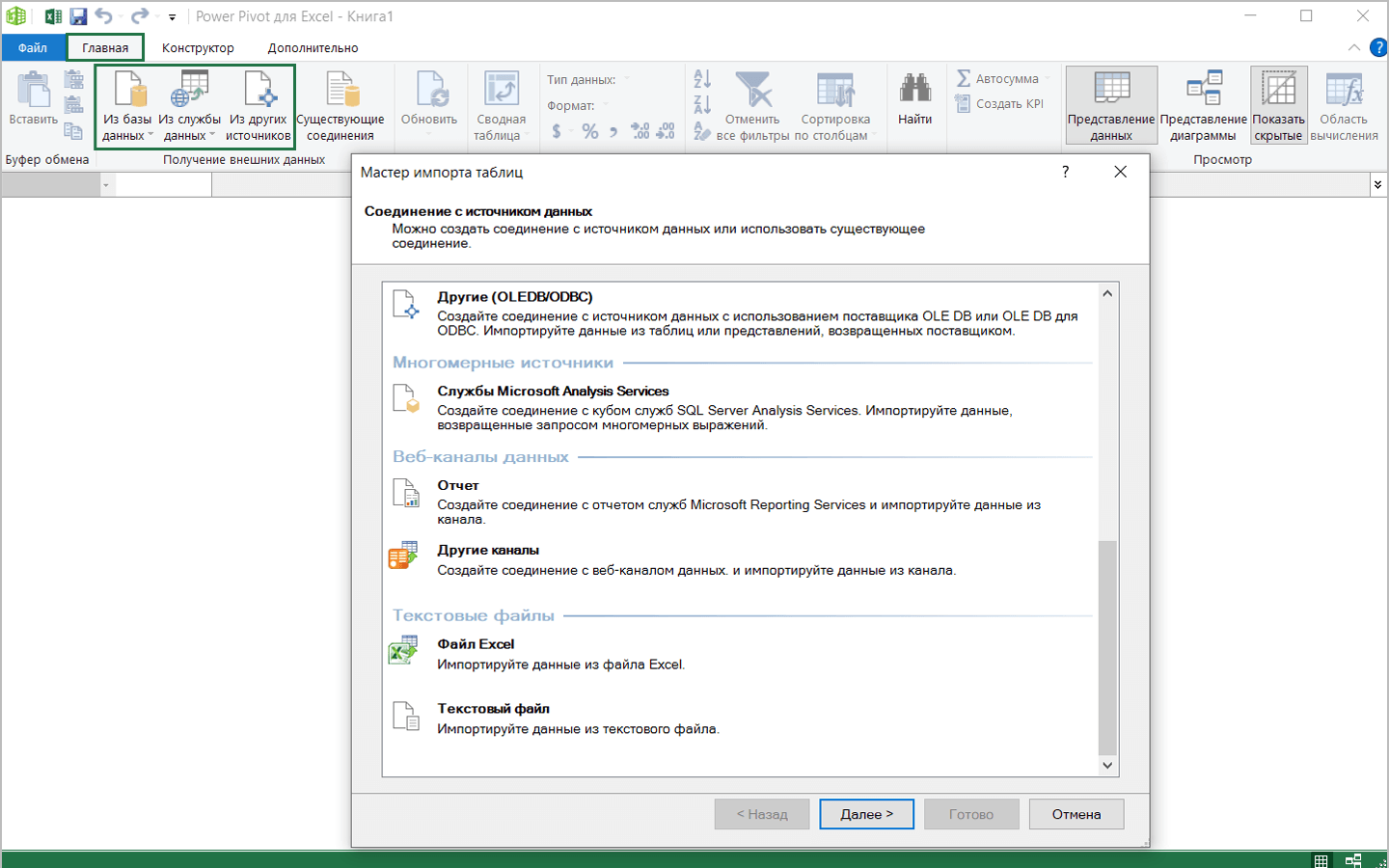
С помощью встроенных инструментов настраивается подключение к 15 видам источников данных.
Увидеть весь список можно в окне «Мастер импорта таблиц», которое открывается в меню Главная → Из других источников.
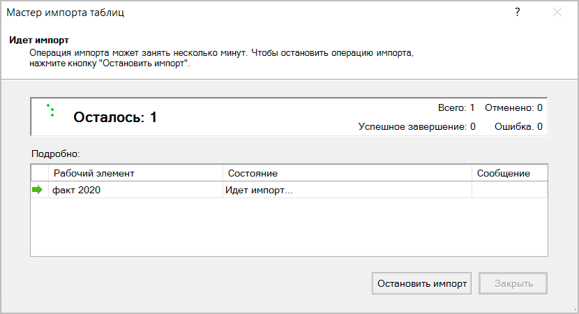
Настроим подключение к данным на примере файла Excel. Укажите путь к файлу, поставьте галочку «Использовать первую строку в качестве заголовков столбцов», выберите таблицы, жмем «Готово». У вас в окне включится счетчик импорта строк — работает довольно быстро. В результате импорта в окне Power Pivot появятся вкладки с таблицами.
Способ 2. Добавить данные из Power Query.
Загрузка данных с помощью инструментов Power Pivot делается легко, но Power Query лучше подходит для импорта и значительно расширяет возможности аналитики. В нем намного больше доступных источников и возможностей для обработки таблиц произвольного вида.
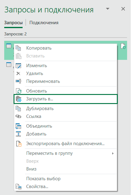
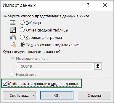
Чтобы настроить подключение с помощью Power Query, вам нужно создать запрос к источнику данных. Список ранее созданных запросов находится на вкладке «Запросы и подключения». Нажмите на запрос правой кнопкой мышки и выберите Загрузить в… В открывшемся окне доступных вариантов импорта поставьте галочку «Добавить эти данные в модель данных». Задать настройки импорта также можно в самом редакторе Power Query.
К сожалению, в Excel 2010 Power Pivot почти невозможно «подружить» с Power Query и этот новый функционал в старом Excel сильно ограничен.
Интерфейс Power Pivot
Разберем подробнее интерфейс Power Pivot.
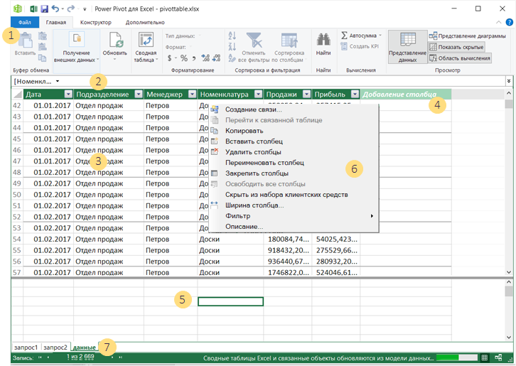
В окне Power Pivot есть:
- Лента редактора для вкладок меню Главная, Конструктор, Дополнительно.
- Строка формул на языке DAX.
- Область данных и вычисляемых столбцов.
- Добавление нового вычисляемого столбца.
- Область вычислений, в которой можно писать меры.
- Меню, которое появляется при нажатии правой кнопкой мышки.
- Ярлычки с названиями таблиц данных для переключения между ними (как между листами в «обычном» Excel).
Модель данных и связи
Чтобы перейти к настройке связей между таблицами, выберите в меню Главная → Представление диаграммы (вернутся обратно к просмотру таблиц можно, нажав Представление данных).

Модель данных в Power Pivot – это набор таблиц, объединенных связями.
Графически связь таблиц обозначается линией между ними, как в примере на рисунке. Чтобы создать связь, выделите мышкой поле в одной таблице и «перетащите» его на соответствующее ему поле в области другой таблицы.

Power Pivot поддерживает типы связей «один к одному», «один ко многим».
- Понять, какой именно вид связи задан между таблицами, можно с помощью значков на концах линий: на стороне «один» стоит символ единица — «1», а на стороне «многие» — звездочка «*». Если между таблицами задана связь «один к одному», то на концах линии будут единички «1».
- Поля, которые используются для создания связей, называются ключами связи. В таблицах, которые находятся на стороне «один» (конец линии с единичкой «1») в ключевых столбцах должны содержаться только уникальные значения. В таблицах на стороне «многие» со звездочкой «*» в ключевых столбцах те же значения, но они могут повторяться много раз.
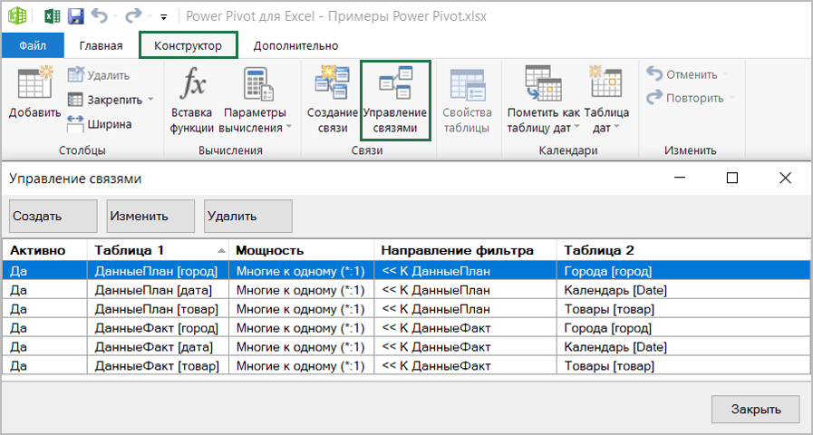
- Стрелка на линии связи обозначает направление фильтрации. Так, на рисунке выше справочники Товары и Города фильтруют таблицы ДанныеФакт и ДанныеПлан.
Если выделить мышкой линию связи в модели данных, то можно увидеть, с помощью каких полей задана связь. Выделенные линии можно удалять. Или, щелкнув по ним дважды, менять связи в открывшемся окне. Также управление связями доступно в окне, которое открывается в меню Конструктор → Управление связями.
Вычисления в Power Pivot
Формулы Power Pivot пишут на языке DAX (Data Analysis Expressions, выражения для анализа данных). DAX-формулы позволяют, по аналогии с формулами Excel, выполнять вычисления и/или настраивать произвольную фильтрацию и представление данных в таблицах.
Язык DAX впервые появился в 2010 году вместе с надстройкой Power Pivot. В этом языке сотни функций, с помощью которых можно создавать аналитические расчеты. Кроме Power Pivot в Excel, DAX-формулы также доступны в Power BI и Analysis Services. То есть эти формулы вам точно пригодятся.
Вычисления с помощью DAX-формул создаются в виде:
- вычисляемых столбцов, как в обычных таблицах Excel.
- мер, которые пишут в области вычислений под таблицей.
Вычисляемые столбцы представляют собой столбцы в таблицах данных, созданные с помощью формул. Чтобы добавить такой столбец, щелкните мышкой дважды по столбцу слева «Добавление столбца», введите название вычисления, а затем знак «=» и формулу в строке формул.
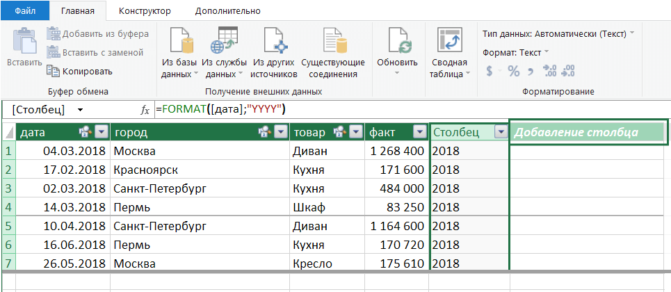
Вычисляемый столбец похож на любой другой столбец в таблице. Также с помощью таких столбцов можно создавать связи в модели. Вычисляемые столбцы в Excel рассчитываются в момент загрузки (обновления) данных, а значения в самом столбце сохраняются, увеличивая размер файла. То есть столбцы – это статические вычисления.
Как и вычисляемые столбцы, меры тоже создаются с помощью DAX-формул. В отличие от столбцов, меры – это динамические вычисления, результат которых зависит от контекста – его можно увидеть в отчете, где мы задаем в разрезе каких полей, фильтров и др. вычислить меру. Меры записываются под таблицей в области вычислений.
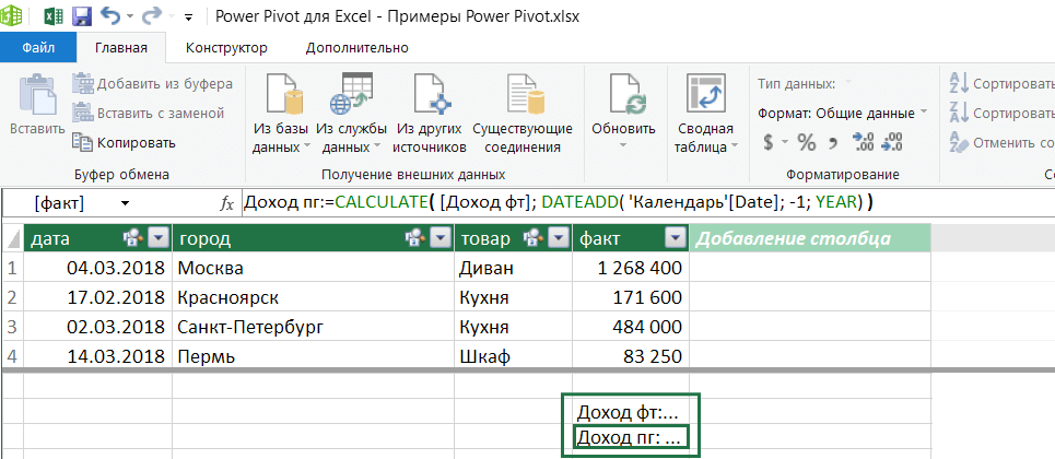
Меры в Power Pivot можно превратить в KPI – ключевые показатели эффективности. Для этого выделите меру и нажмите на кнопку Создать KPI в меню Главная. Кроме мер, созданных пользователями, в Excel также есть неявные меры. Они создаются автоматически при формировании сводной таблицы, когда пользователь помещает данные в область значений. Чтобы посмотреть, есть ли у вас в Power Pivot неявные меры, выберите на вкладке Главная → Показать скрытые.
Подробнее о DAX-формулах:
- Основные формулы Power Pivot
- ТОП-20 DAX формул для Power Pivot и Power BI
Power Pivot for Excel Tutorial: Top Use Cases and Examples
With the arrival and growing ubiquity of big data, Excel, as a data-mining and processing tool has been pushed to its limits—reflected in its dated 1,048,576 row hard limit and the application’s processing speed slowing to a crawl. As of 2010, Microsoft released a Power Pivot function that transformed the scope and usefulness of Excel where the extraction, combination, and analysis of large datasets are concerned.
Using live cases, Finance Expert Ellen Su explores in detail how to master Power Pivot and explores its hidden advantages as a big data tool.
authors are vetted experts in their fields and write on topics in which they have demonstrated experience. All of our content is peer reviewed and validated by Toptal experts in the same field.
With the arrival and growing ubiquity of big data, Excel, as a data-mining and processing tool has been pushed to its limits—reflected in its dated 1,048,576 row hard limit and the application’s processing speed slowing to a crawl. As of 2010, Microsoft released a Power Pivot function that transformed the scope and usefulness of Excel where the extraction, combination, and analysis of large datasets are concerned.
Using live cases, Finance Expert Ellen Su explores in detail how to master Power Pivot and explores its hidden advantages as a big data tool.
authors are vetted experts in their fields and write on topics in which they have demonstrated experience. All of our content is peer reviewed and validated by Toptal experts in the same field.

By Ellen Su
Verified Expert in Finance
Ellen’s extensive experience in fixed income trading and portfolio management make her an unparalleled expert in analytics and modeling.
Expertise
Previously At
Read the Spanish version of this article translated by Marisela Ordaz.
Executive Summary
- Introduced to Excel 2010 and 2013 as an add-on, but now native to the application, Power Pivot is part of Microsoft’s business intelligence stack capable of (but not limited to) big data analytics work without specialty infrastructure or software.
- According to Microsoft, «Power Pivot enables you to import millions of rows of data from multiple data sources into a single Excel workbook, create relationships between heterogeneous data, create calculated columns and measures using formulas, build PivotTables and PivotCharts, and further analyze the data so that you can make timely business decisions without requiring IT assistance.»
- Power Pivot was created in direct response to the big data demands of contemporary business intelligence needs, which prior generations of Excel—given their 1,048,576 row limit or processing speed shortcomings—struggled to cope with.
- Power Pivot is expressed by Microsoft using DAX (Data Analysis Expressions), which is a collection of functions, operators, and constants usable in a formula or expression to calculate/return one or more values.
- Power Pivot lets you import and manipulate hundreds of millions of rows of data whereas Excel has a hard constraint of just over a million rows.
- Power Pivot allows you to import data from multiple sources into one single source workbook without having to create multiple source sheets and deal with potential version control and transferability issues.
- Power Pivot lets you manipulate the imported data, analyze it, and draw conclusions without slowing down your computer system, as is typical of Basic Excel.
- Power Pivot lets you visualize and manipulate your big datasets with PivotCharts and Power BI, where basic Excel lacks these capabilities.
- By working alongside you as a thought partner to design, structure, build, and deliver a range of financial models, budgets, and big-data analyses/projects, all en route to decisions around captive projects, mergers and acquisitions, or strategic investments.
- By creating customized models unique to your business, using Power Pivot and other specialty excel functions.
- By also creating prefabricated, go-to templates that can be adapted uniquely by almost anyone across your organization, for almost any purpose, using Power Pivot and other specialty Excel functions.
- By training individuals or groups within your organization on everything from the basics of excel, modeling and analysis to advanced quantitative methods using Power Pivot, Power Pivot tables, Power Pivot charts, and PowerQuery.
- By actualizing each of these and more, alongside the design, creation, and delivery of a polished and professional PowerPoint presentation, ahead of strategic decisions.
Download the data set here to follow along with the tutorial.
The Emperor’s New Clothes: Excel Power Pivot Tutorial
Across the various fields and sub-sub-fields that span finance, financial analysis, financial markets, and financial investing, Microsoft Excel is king. With the arrival and exponential growth of big data, however, driven by decades of data aggregation and accumulation, the advent of cheap cloud storage and the rise of the internet of things—i.e., eCommerce, social media, and the interconnectedness of devices—Excel’s legacy functionality and capabilities have been pushed to their limits.
More specifically, older-generation Excel’s infrastructure and processing limitations such as its row-limit of 1,048,576 rows, or inevitable processing slow-down where large data sets, data tables and interconnected spreadsheets are concerned, reduced its usability as a effective big data tool. In 2010 however, Microsoft added a new dimension to Excel, called Power Pivot. Power Pivot offered next-generation business intelligence and business analytics functionality to Excel in its ability to extract, combine, and analyze almost limitless datasets without processing speed impairment. Despite its release eight years ago, however, most financial analysts still do not know how to use Excel Power Pivot, and many do not know it even exists.
In this article, I will show you how to use Power Pivot basics to overcome common Excel issues and take a look at additional key advantages of the software using some examples. This Power Pivot tutorial is meant to serve as a guide for what you can achieve with this tool, and at the end, it will explore some sample use-cases where Power Pivot often proves invaluable.
What Is Power Pivot and Why Is It Useful?
Power Pivot is a feature of Microsoft Excel that was introduced as an add-in to Excel 2010 and 2013, and is now a native feature for Excel 2016 and 365. As Microsoft explains, Power Pivot for Excel “enables you to import millions of rows of data from multiple data sources into a single Excel workbook, create relationships between heterogeneous data, create calculated columns and measures using formulas, build PivotTables and PivotCharts, and then further analyze the data so that you can make timely business decisions without requiring IT assistance.”
The primary expression language that Microsoft uses in Power Pivot is DAX (Data Analysis Expressions), although others can be used in specific situations. Again, as Microsoft explains, “DAX is a collection of functions, operators, and constants that can be used in a formula, or expression, to calculate and return one or more values. Stated more simply, DAX helps you create new information from data already in your model.” Fortunately for those already familiar with Excel, DAX formulas will look familiar, since many of the formulas have a similar syntax (e.g., SUM , AVERAGE , TRUNC ).
For clarity, the key benefits of using Power Pivot vs. basic Excel can be summarized as the following:
- It lets you import and manipulate hundreds of millions of rows of data where Excel has a hard constraint of just over a million rows.
- It allows you to import data from multiple sources into one single source workbook without having to create multiple source sheets that suffer from version control and transferability issues.
- It lets you manipulate the imported data, analyze it, and draw conclusions without slowing down your computer to a snail’s pace.
- It lets you visualize the data with PivotCharts and Power BI.
In the following sections, I’ll run through each of the above and show you how Power Pivot for Excel can be helpful.
How to Use Power Pivot
1) Importing Large Datasets
As previously alluded to, one of the major limitations of Excel pertains to working with extremely large datasets. Fortunately for us, Excel can now load well over the one-million row limit directly into Power Pivot.
To demonstrate this, I generated a sample dataset of two years’ worth of sales for a sporting goods retailer with nine different product categories and four regions. The resulting dataset is two million rows.
Using the Data tab on the ribbon, I created a New Query from the CSV file (see Creating a New Query below). This functionality used to be called PowerQuery, but as of Excel 2016 and 365, was more tightly integrated into the Data tab of Excel.
From a blank workbook in Excel to loading all two million rows into Power Pivot, it took about one minute! Notice that I was able to perform some light data formatting by promoting the first row to become the column names. Over the past few years, the Power Query functionality has vastly improved from an Excel add-in to a tightly integrated part of the Data tab on the toolbar. Power Query can pivot, flatten, cleanse, and shape your data through its suite of options and its own language, M.
2) Importing Data from Multiple Sources
One of the other key benefits of Power Pivot for Excel is the ability to easily import data from multiple sources. Previously, many of us created multiple worksheets for our various data sources. Often, this process involved writing VBA code and copy/pasting from these disparate sources. Fortunately for us, though, Power Pivot allows you to import data from different data sources directly into Excel without having to run into the issues mentioned above.
Using the Query function in Exhibit 1, we can pull from any of the following sources:
- Microsoft Azure
- SQL Server
- Teradata
- Salesforce
- JSON files
- Excel workbooks
- …and many more
Further, multiple data sources can be combined either in the Query function or in the Power Pivot window to integrate data. For example, you can pull production-cost data from an Excel workbook and actual sales results from SQL server through the Query into Power Pivot. From there, you can combine the two datasets by matching production-batch numbers to produce per-unit gross margins.
3) Working with Large Datasets
Another key advantage of Power Pivot in Excel is the ability to manipulate and work with large datasets to draw relevant conclusions and analysis. I’ll run through a few common examples below to give you a sense of the power of the tool.
Measures
Excel junkies will no doubt agree that PivotTables are both one of the most useful, and at the same time, one of the most frustrating tasks we perform. Frustrating particularly when it comes to working with larger data sets. Fortunately, Power Pivot for Excel allows us to easily and quickly create PivotTables when working with larger sets of data.
In the image below, entitled Creating Measures, notice how the Power Pivot window is separated into two panes. The top pane has the data, and the bottom pane houses the measures. A measure is a calculation that is performed across the entire dataset. I have entered a measure by typing in the highlighted cell.
Total Sales:=SUM('Accounting Data'[Amount])This creates a new measure that sums across the Amount column. Similarly, I can type another measure in the cell below
Average Sales:=AVERAGE('Accounting Data'[Amount])
From there, watch how quickly it is to create a familiar PivotTable on a large dataset.
Dimension Tables
As financial analysts using Excel, we become adept at using convoluted formulas to bend the technology to our will. We master VLOOKUP , SUMIF , and even the dreaded INDEX(MATCH()) . However, by using Power Pivot, we can throw much of that out the window.
To demonstrate this functionality, I created a small reference table in which I assigned each Category to a Type. By choosing “Add to Data Model,” this table is loaded into Power Pivot (see Adding a User-created Table to a Power Pivot Model above).
I also created a date table to use with our dataset (see Creating a Date Table below). Power Pivot for Excel makes it easy to create a date table quickly in order to consolidate by months, quarters, and days of the week. The user can also create a more custom date table to analyze by weeks, fiscal years, or any organization-specific groupings.
Calculated Columns
Besides measures, there is another type of calculation: calculated columns. Excel users will be comfortable writing these formulas, as they are very similar to writing formulas in data tables. I have created a new calculated column below (see Creating a Calculated Column below) which sorts the Accounting Data table by Amount. Sales below $50 are labeled “Small,” and all others are labeled “Large.” Doesn’t the formula feel intuitive?
Relationships
We can then create a relationship between the Accounting Data table’s Category field and the Category table’s Category field using the Diagram View. Additionally, we can define a relationship between the Accounting Data table’s Sales Date field and the Calendar table’s Date field.
Now, without any SUMIF or VLOOKUP functions needed, we can create a PivotTable that calculated Total Sales by year, and type, with a slicer for Transaction Size.
Or, we can create a chart of Average Sales for each day of the week using the new Calendar table.

While this chart looks simple, it is impressive that it took less than ten seconds to create a consolidation over two million rows of data, without adding a new column to the sales data.
While being able to perform all these consolidated reporting scenarios, we can always still drill down into the individual line items. We retain our highly granular data.
Advanced Functions
So far, most of the analysis I have shown are relatively straightforward calculations. Now, I want to demonstrate the some of the more advanced capabilities of this platform.
Time Intelligence
Often, when we examine financial results, we want to compare it to a comparable timeframe from the previous year. Power Pivot has some built-in time intelligence functions.
Same Period Last Year Sales:=CALCULATE([Total Sales],SAMEPERIODLASTYEAR('Calendar'[Date])) YOY Sales Growth:=if(not(ISBLANK([Same Period Last Year Sales])),([Total Sales]/[Same Period Last Year Sales])-1,BLANK())For example, adding just two measures above to the Accounting Data table in Power Pivot enables me to produce the following PivotTable in a few clicks.

Mismatched Granularities
As a financial analyst, one problem I often have to solve is that of mismatched granularities. In our example, the actual sales data is shown to the category level, but let’s prepare a budget that is only on a seasonal level. To further this mismatch, we will prepare a quarterly budget, even through the sales data is daily.

With Power Pivot for Excel, this inconsistency is easily solved. By creating two additional reference tables, or dimension tables in database nomenclature, we can now create the appropriate relationships to analyze our actual sales against the budgeted amounts.

In Excel, the following PivotTable comes together quickly.

Further, we can define new measures that calculate the variance between actual sales and budgeted sales as below:
Actual-to-Budget Variance:=DIVIDE([Total Sales],[Total Budgeted Sales])-1Using this measure, we can show the variance on a PivotTable.

Percent of Total
Finally, let’s examine sales in a particular category as a percent of all sales (e.g., category contribution to overall sales), and sales in a particular category as a percent of all sales of the same type (e.g., category contribution to seasonal-type sales). I created the two measures below:
Total Sales as Percent of All Sales:=[Total Sales]/CALCULATE([Total Sales],ALL('Accounting Data')) Total Sales as Percent of Type:=[Total Sales]/CALCULATE([Total Sales],ALL('Accounting Data'[Category]))Those measures can now be deployed in a new PivotTable:

Notice how the calculations are performed at both the category and seasonal type level. I love how quickly and effortlessly these calculations are performed on such a large dataset. These are just a few examples of the elegance and sheer computational power of Power Pivot.
Compression
Another benefit is that file sizes shrink. The original file size was 91MB, and now it is under 4MB. That is a compression of 96% of the original file.

How does this happen? Power Pivot uses the xVelocity engine to compress the data. In simple terms, the data is stored in columns rather than rows. This storage method allows the computer to compress duplicate values. In our example dataset, there are only four regions that are repeated over all two million rows. Power Pivot for Excel can more efficiently store this data. The result is that for data that have many repeating values, it costs much less to store this data.
One thing to note is that I used whole-dollar amounts in this sample dataset. If I had included two decimal points to reflect cents, the compression effect would lessen to a still-impressive 80% of the original file size.
SSAS Tabular
Power Pivot models can also be scalable to the entire enterprise. Let’s say you build a Power Pivot model that starts gaining many users in the organization, or the data grows to ten million rows, or both. At this point, you may not want thirty different users refreshing the model or making changes. The model can be seamlessly converted into SSAS Tabular. All the tables and relationships are retained, but now you can control the refresh frequency, assign roles (e.g., read-only, read and process) to various users, and deploy only a small Excel front-end which links into the Tabular model. The result is that your users could then access the deployed Tabular model with a small workbook, but not have access to the formulas and measures.
4) Data Visualization and Analysis
CUBE Formulas
One of the constant requests of my clients is that I create reporting that conforms to a strictly defined layout. I have clients that request specific column widths, RGB color codes, and pre-defined font names and sizes. Consider the following dashboard:

How do we populate the sales numbers without generating PivotTables if all of our sales are housed with Power Pivot for Excel? Using CUBE formulas! We can write CUBE formulas within any Excel cell and it will perform the calculation using the Power Pivot model we have already constructed.
For example, the following formula is typed in the cell under “2016 Total Sales:”
=CUBEVALUE("ThisWorkbookDataModel","[Measures].[Total Sales]","[Calendar].[Year].[2016]")The first part of the formula, highlighted in yellow, refers to the name of the Power Pivot model. In general, it is usually ThisWorkbookDataModel for newer versions of Power Pivot for Excel. The portion in green defines that we want to use the measure Total Sales. The part in blue instructs Excel to filter for only rows that have a Sales Date with a year equal to 2016.
Behind the scenes, Power Pivot has constructed an Online Analytical Processing (OLAP) cube with the data, calculated columns, and measures. This design allows the Excel user to then access the data by fetching directly with the CUBE functions. Using CUBE formulas, I have been able to construct full financial statements that conform to predefined layouts. This capability is one of the highlights of using Power Pivot for Excel for financial analysis.
Power BI
Another advantage of Power Pivot for Excel is that you can quickly take any Power Pivot workbook you build and quickly convert it into a Power BI model. By importing the Excel workbook directly into the Power BI Desktop app or Power BI Online, you can analyze, visualize, and share your data with anyone in your organization. Essentially, Power BI is Power Pivot, PowerQuery, and SharePoint all rolled into one. Below, I have created a dashboard by importing the previous Power Pivot for Excel workbook into the Power BI desktop application. Notice how interactive the interface is:
One great thing about Power BI is the Natural Language Q&A. To demonstrate, I uploaded the Power BI model onto my online Power BI account. From the website, I can ask questions and Power BI constructs the appropriate analysis as I type:
This type of query ability enables the user to ask questions of the data model and interact with the data in an easier way than in Excel.
Another benefit of Power BI is that the developers at Microsoft are constantly releasing updates to it. New features, many user-requested, are pushed out monthly. Best of all, it is a seamless transition from Power Pivot for Excel. So, the time you invested learning the DAX formulas can be deployed in Power BI! For the analyst who needs to share his analysis to many users on varying devices, Power BI may be worth exploring.
Best Practices
Once you get started, there are a few best practices that you should follow.
The first is to thoughtfully decide what to import in the first place. Will you ever use the salesperson’s home address? Do I need to know my customer’s email address in the context of this workbook? If the goal is to aggregate the data into a dashboard, then some of the data that is available will not be necessary for those calculations. Spending time curating the data coming in will greatly alleviate issues and memory-usage later when your dataset expands.
Another best practice is to remember that Power Pivot is not Excel. In Excel, we are accustomed to creating calculations by constantly expanding our worksheets to the right. Power Pivot for Excel most efficiently processes the data if we limit this desire for manifest destiny. Instead of continuously creating calculated columns to the right of your data, learn to write measures in the bottom pane. This habit will ensure smaller file sizes and quicker computations.
Finally, I would suggest using plain-English names for measures. This one took me a long time to adopt. I spent the first few years making up names like SumExpPctTotal , but once other people began to use the same workbooks, I had a lot of explaining to do. Now, when I start a new workbook, I use measure names like Expense Line Item as Percent of Total Expenses . While the name is longer, it is much easier for someone else to use.
Real-World Use Cases
In this article I have presented only a handful of the ways in which Power Pivot for Excel allows you to take an important step beyond plain-vanilla Excel. I thought it would be useful to highlight some real-world use cases in which I’ve found Power Pivot for Excel is extremely useful.
- Analyze performance of a large portfolio of assets over varying time ranges: Since Power Pivot for Excel allows us to define measures that compare a time-period with a previous one, we can quickly have quarter-over-quarter, year-over-year, and month-over-month performance all on a rolling basis by writing only a few measures.
- Summarize accounting data using customized aggregation levels: By identifying each general-ledger line item by name, category, and financial statement, reports can quickly be created that include the appropriate line items.
- Chains can identify same-store sales: Using a table that maps when stores come online, financial results can be compared on a same-store basis.
- Pinpoint over- and under-performers in sales: PivotTables can be created that highlight the top five SKUs and bottom five SKUs by sales, gross margins, production timeframes, etc.
- Retailers can define calendar tables that use a 4-4-5 configuration: Using a custom date table, a retailer can assign each day to a specific 4-4-5 month easily, then daily sales results can be rolled into the corresponding month.
From Clunky Spreadsheets to Modern Workbooks
As financial analysts, we are required to perform complex calculations on ever-expanding datasets. Since Excel is already the default analytical tool, the Power Pivot learning curve is easy, and many of the functions mirror Excel’s native functions.
With the use of CUBE functions, Power Pivot for Excel seamlessly blends into your existing Excel workbooks. The computational efficiency gain cannot be overlooked. Assuming a 20% faster processing speed, which is conservative, the financial analyst that spends six hours a day within Excel can save 300 hours a year!
Additionally, we can now analyze datasets that are much larger than we could previously with our traditional Excel. With models designed efficiently, we can easily have 10x the amount of data that we previously were allowed in traditional Excel, while maintaining quick analytical agility. With the ability to convert the models from Power Pivot to SSAS Tabular, the amount of data that can be processed is 100–1,000 times what we can achieve in Excel.
Power Pivot for Excel’s ability to perform lightning-fast calculations on large amounts of data and still retain the ability to dive into the details can transform financial analysis from clunky spreadsheets to modern workbooks.
If you’re interested in trying Power Pivot for Excel out, below are some useful materials to get you started.
Useful References and Guides
Collie, R., & Singh, A. (2016). Power Pivot and Power BI: The Excel user’s guide to DAX, Power Query, Power BI & Power Pivot in Excel 2010-2016. United States: Holy Macro! Books.
Ferrari, A., & Russo, M. (2015). The definitive guide to DAX: Business intelligence with Microsoft Excel, SQL Server Analysis Services, and Power BI. United States: Microsoft Press, USA.
Further Reading on the Toptal Blog:
- Exploring Excel’s Get & Transform Functionality
- Product Strategy: A Guide to Core Concepts and Processes
- An Intro to SQL Window Functions
- Design Problem Statements: What They Are and How to Frame Them
- Bridgewater’s Ray Dalio: Quiet Pioneer of Big Data, Machine Learning, and Fintech
Understanding the basics
What is a Power Pivot table?
When you’re looking at Power Pivot vs. Pivot tables, Power Pivot is an Excel feature that enables the import, manipulation, and analysis of big data without loss of speed/functionality. Power Pivot tables are pivot tables that that allow the user to mix data from different tables, affording them powerful filter chaining when working on multiple tables.
How do I create a Power Pivot table?
First, import your dataset into your Power Pivot workbook. Next, in the Power Pivot window on the Power Pivot Home tab, click PivotTable. Next, select “New Worksheet” (Excel will add an empty PivotTable). Then, select the empty PivotTable and follow the instructions detailed there.
How do I create a Power Pivot chart?
First, import your dataset into your Power Pivot workbook. Next create a Power Pivot table. Then, on the Power Pivot tab, click the arrow below PivotTable and select PivotChart. Select “Existing Worksheet” and click “OK.” Excel will add an empty PivotChart to the same worksheet. Follow the instructions there.
Power Pivot в Excel: как выгрузить данные из внешних источников и собрать их в одну базу
Инструкция со скриншотами. Разбираемся, для чего нужна и как работает надстройка Power Pivot для Excel.

Иллюстрация: Meery Mary для Skillbox Media

Ксеня Шестак
Рассказывает просто о сложных вещах из мира бизнеса и управления. До редактуры — пять лет в банке и три — в оценке имущества. Разбирается в Excel, финансах и корпоративной жизни.
Power Pivot — встроенный инструмент Excel для обработки и анализа больших объёмов данных. С помощью неё в Excel загружают данные из нескольких источников разных форматов, моделируют их в одну базу и работают с ней дальше.
В Power Pivot нет ограничений по количеству строк. Excel позволяет работать только с 1 048 000 строк, а в Power Pivot их может быть гораздо больше. При этом производительность программы не уменьшается.
Поэтому Power Pivot точно пригодится в случаях, когда стандартный Excel не справляется с количеством данных и их форматами.
В статье разберёмся:
- для чего нужна и как работает надстройка Power Pivot;
- как загрузить данные из внешних источников в Power Pivot;
- как смоделировать данные в Power Pivot и создать базу данных;
- как узнать больше о работе в Excel.
При подготовке статьи мы использовали материалы курса Skillbox «Excel + Google Таблицы с нуля до PRO».
Для чего нужна надстройка Power Pivot и как она работает
Как мы сказали выше, Power Pivot расширяет стандартные возможности Excel и позволяет обрабатывать большое количество данных из разных источников.
Power Pivot — бесплатная надстройка для Excel. Для Excel 2010 года её нужно загружать отдельно с сайта Microsoft. Для версий после 2013 года она встроена в стандартную функциональность программы. К сожалению, Power Pivot не предусмотрен для macOS-версии Excel.
Работа в Power Pivot проходит в таком порядке:
- Загружаем данные из разных источников — например, из базы данных Microsoft Access, «1C», из текстовых файлов или электронных таблиц, из интернета.
- Настраиваем связи между загруженными данными — создаём модель данных. Для этого не нужна функция ВПР или другие поисковые функции Excel — в Power Pivot свои инструменты для объединения данных.
- Проводим дополнительные вычисления — при необходимости.
- Power Pivot строит на основе моделей данных необходимые отчёты — в виде сводных таблиц или диаграмм.
В следующих разделах разберём на примере, как загружать данные из внешних источников в Power Pivot, как их моделировать. А также покажем, как на основании этих данных создать отчёт в форме сводной таблицы.
Загружаем данные из внешних источников в Power Pivot
Предположим, у нас есть четыре файла разных форматов:
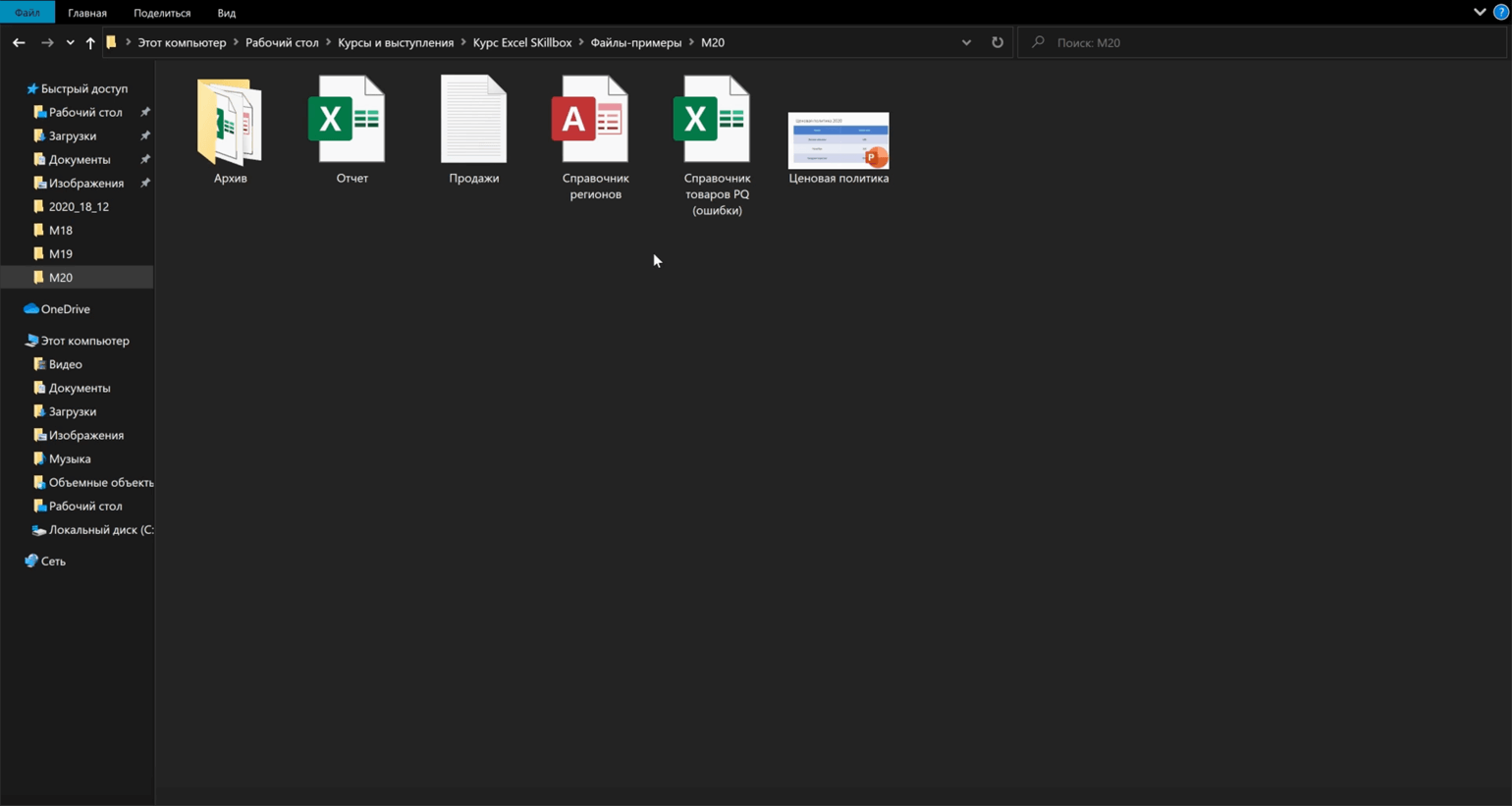
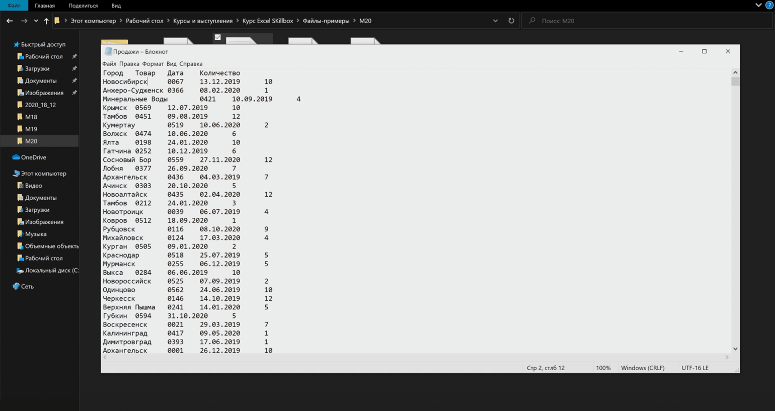
- данные о продажах книжного издательства → в формате TXT;
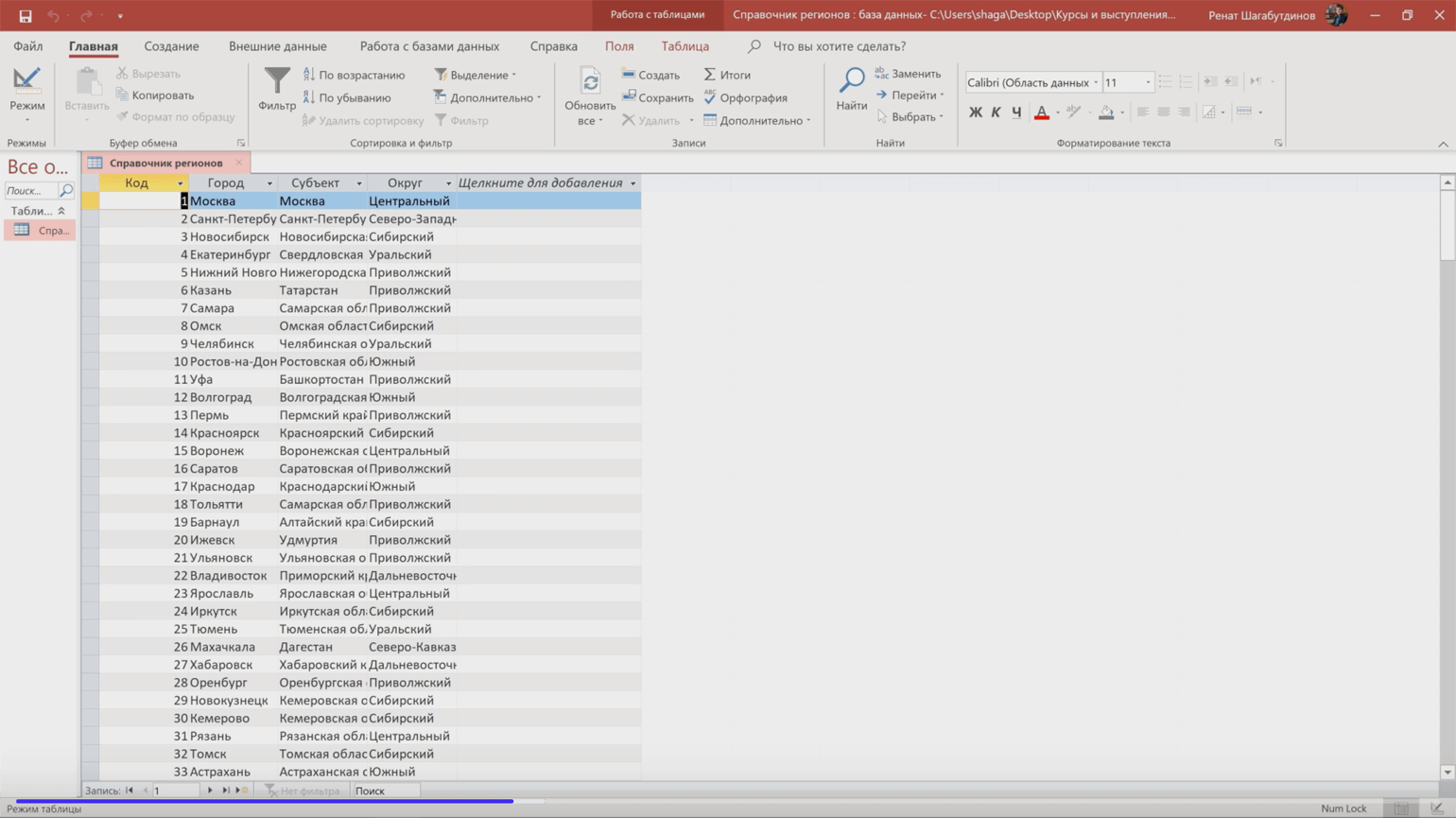
- справочник регионов → в виде базы данных в Access;
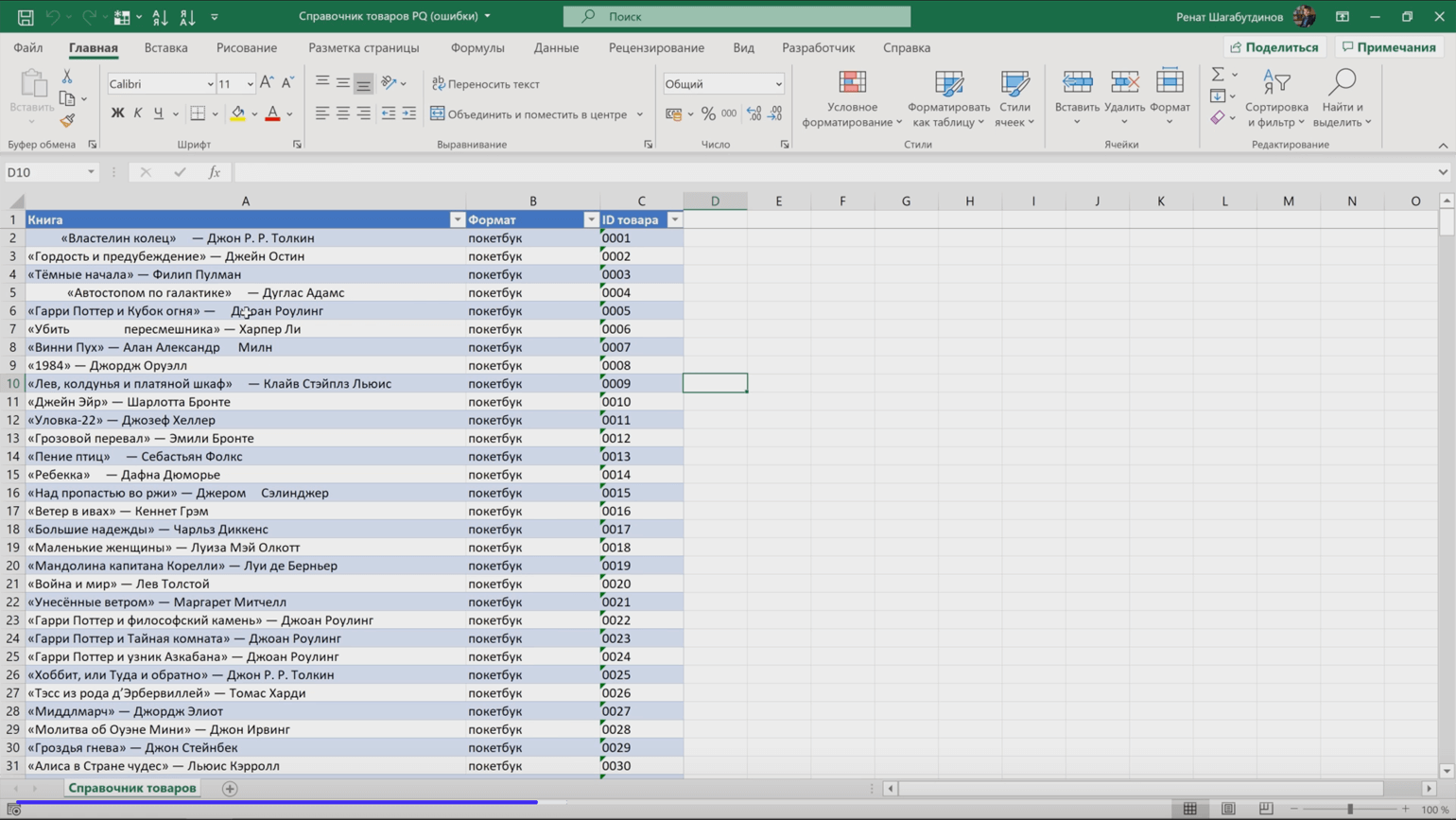
- справочник товаров → в XLS;
- ценовая политика → на слайде Power Point.
Данные о продажах. Это таблица с четырьмя столбцами — город, ID товара, дата продажи и количество проданных единиц — и более чем полутора миллионами строк.
Справочник регионов. В файле одна таблица, в которой перечислены все города России, субъекты и округа.
Справочник товаров. В этой таблице перечислены названия книг, их формат и ID‑номер.
Ценовая политика. Это слайд, где указаны актуальные цены на книги разных форматов.
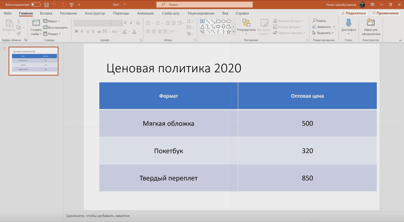
Наша задача — связать данные из этих источников в одну базу. Для начала нужно загрузить эти данные в Power Pivot.
Шаг 1
Открываем пустой файл Excel и активируем надстройку Power Pivot
Для этого потребуется разблокировать вкладку «Разработчик». Переходим во вкладку «Файл» и выбираем пункты «Параметры» → «Настройка ленты». В открывшемся окне в разделе «Основные вкладки» находим пункт «Разработчик», отмечаем его галочкой и нажимаем кнопку «ОК» → в основном меню Excel появляется новая вкладка «Разработчик».
Теперь на этой вкладке нажимаем кнопку «Настройки COM», в появившемся окне выбираем Microsoft Power Pivot for Excel и жмём «ОК».
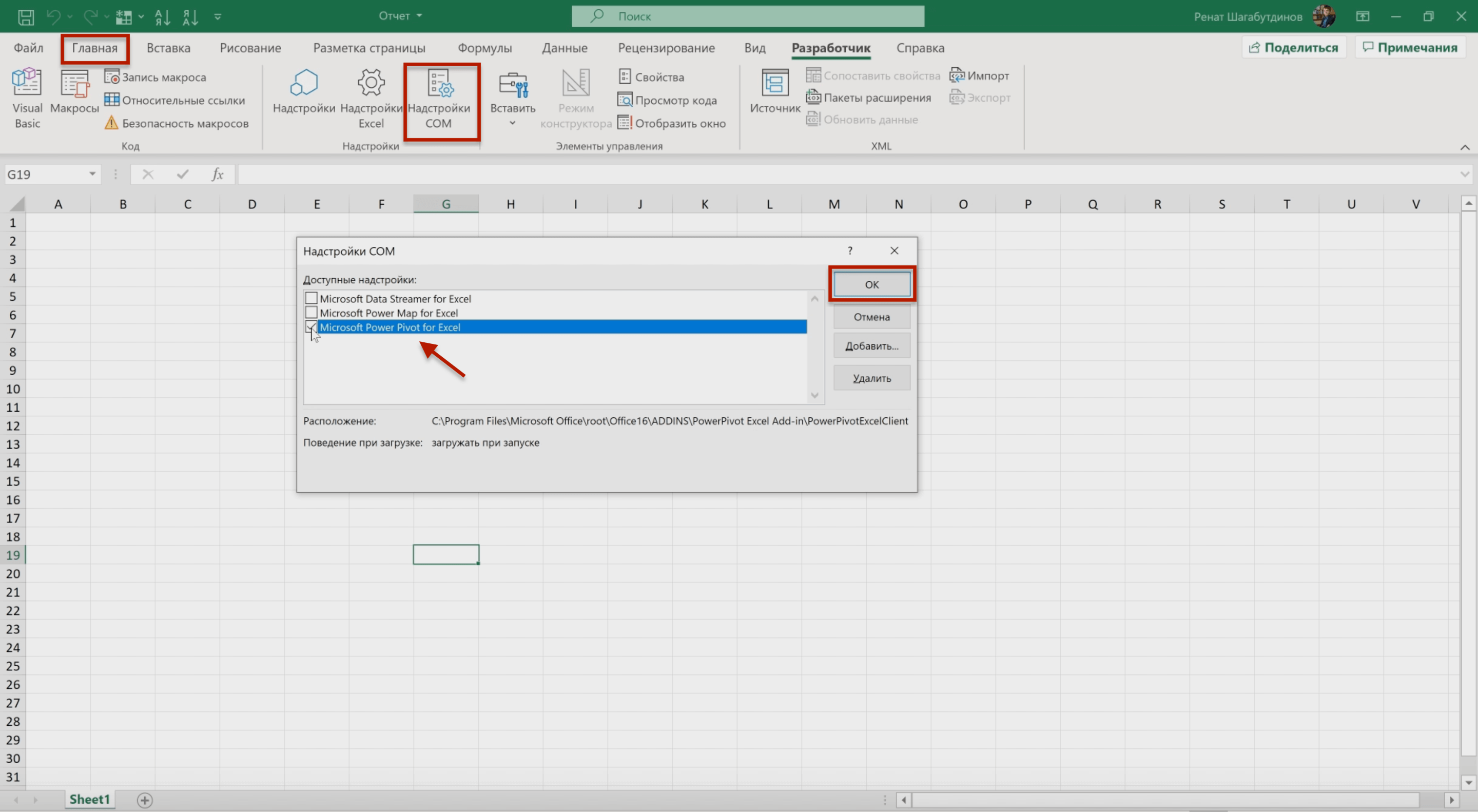
Готово — на панели появилась отдельная вкладка Power Pivot.
Шаг 2
Открываем окно Power Pivot
Для этого переходим на вкладку Power Pivot и нажимаем на кнопку «Управление».
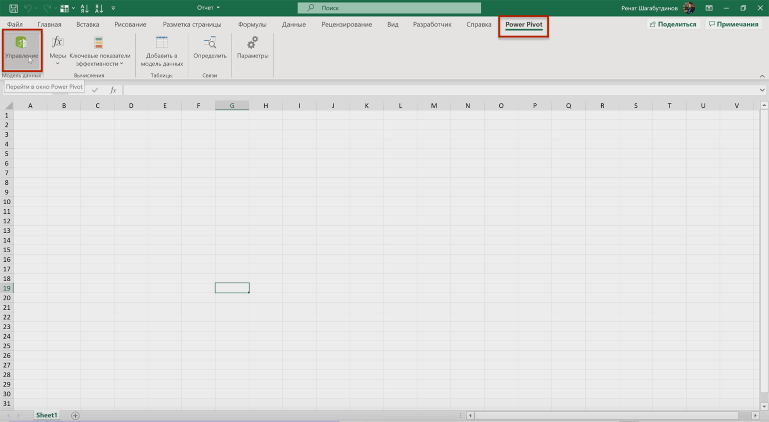
Готово — открылось окно Power Pivot. Оно относится к файлу Excel, через который мы его открыли.
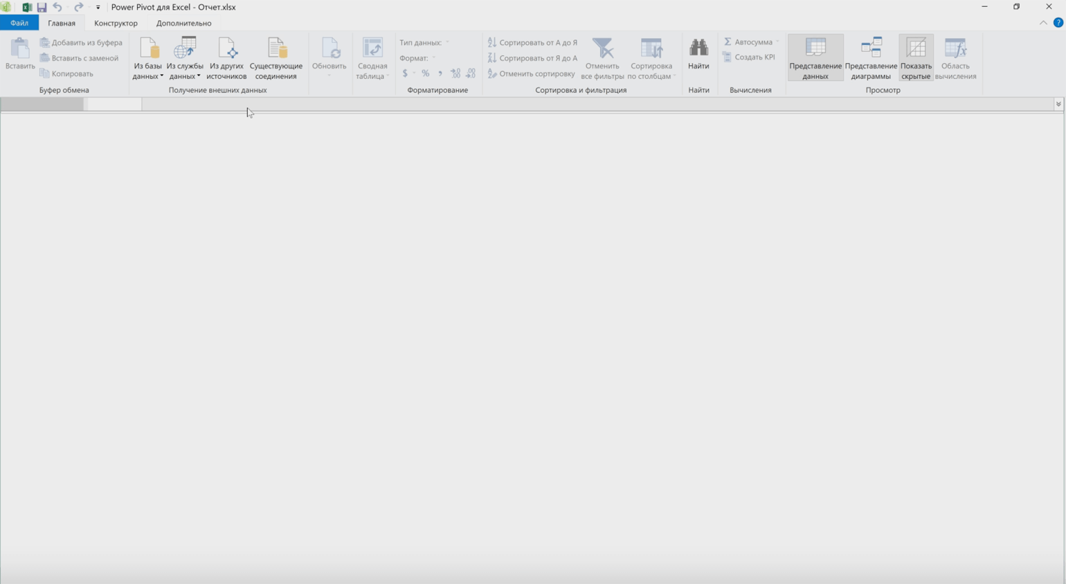
В этом окне нам нужно собрать данные из наших четырёх источников и настроить связи между ними.
Шаг 3
Выгружаем данные из баз данных
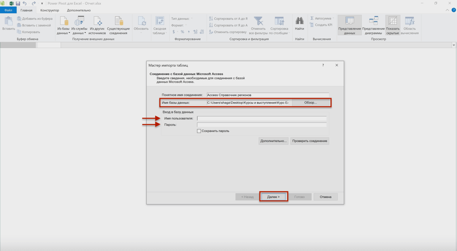
На вкладке «Главная» нажимаем кнопку «Из базы данных» и выбираем «Из Access».

В появившемся окне в поле «Имя базы данных» прописываем адрес, где хранится файл Access со справочником регионов, — адрес можно найти через кнопку «Обзор».
Если база данных зашифрована, в этом же окне нужно ввести имя пользователя и пароль.
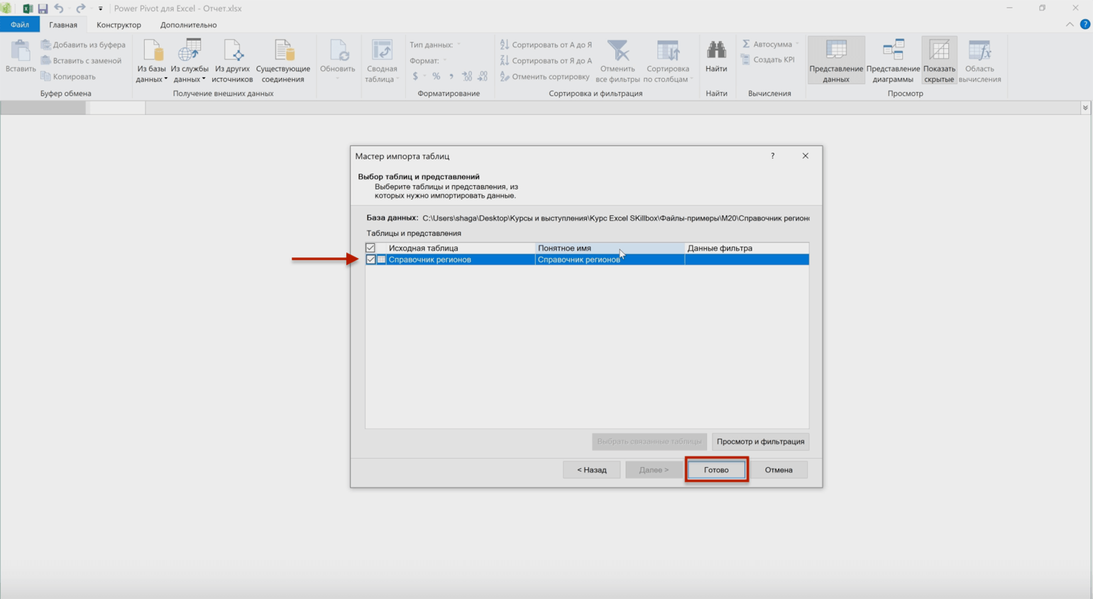
В следующем окне появляется список всех таблиц, которые хранятся в выбранной базе данных.
В нашем случае она одна — «Справочник регионов». Выбираем её и нажимаем «Готово».
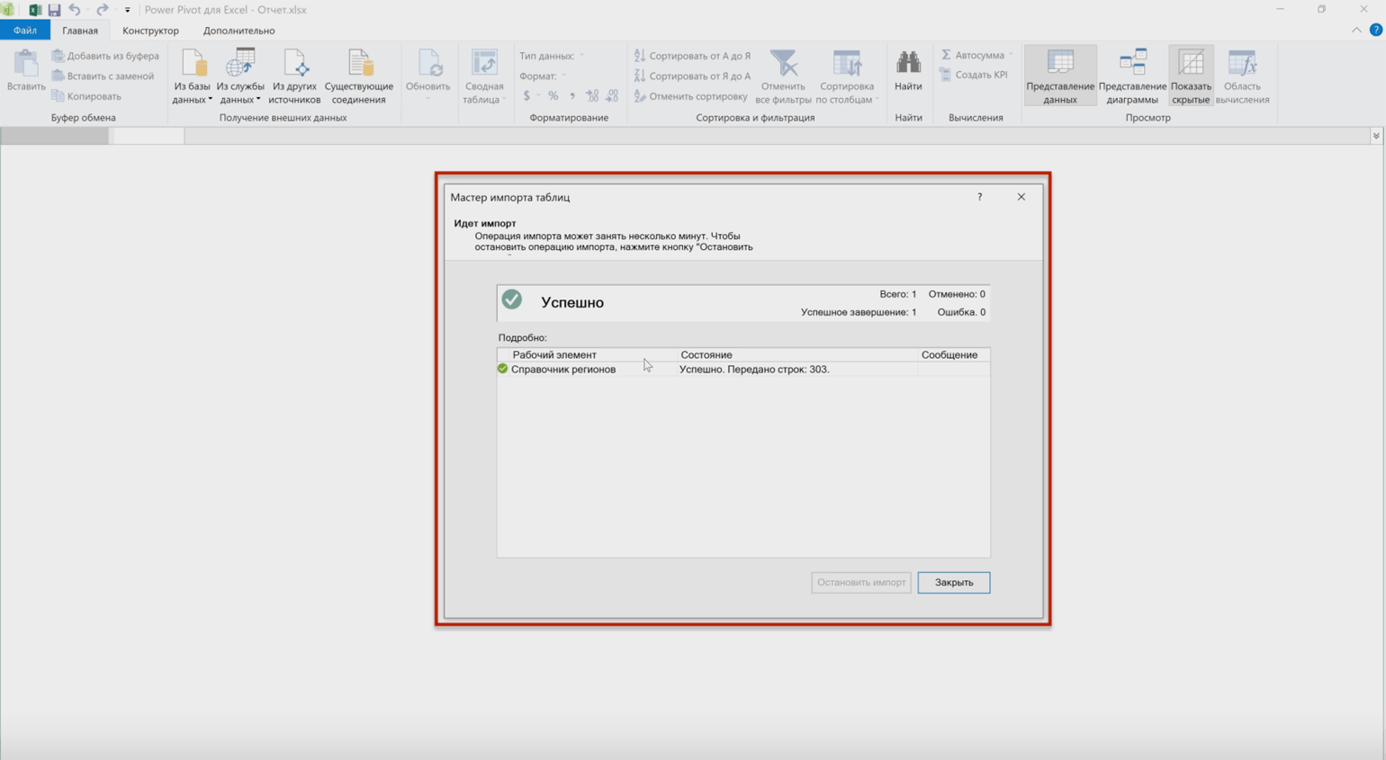
Начинается импорт выбранной таблицы в Power Pivot. После этого появляется окно с результатом. Проверяем информацию и нажимаем «Закрыть».
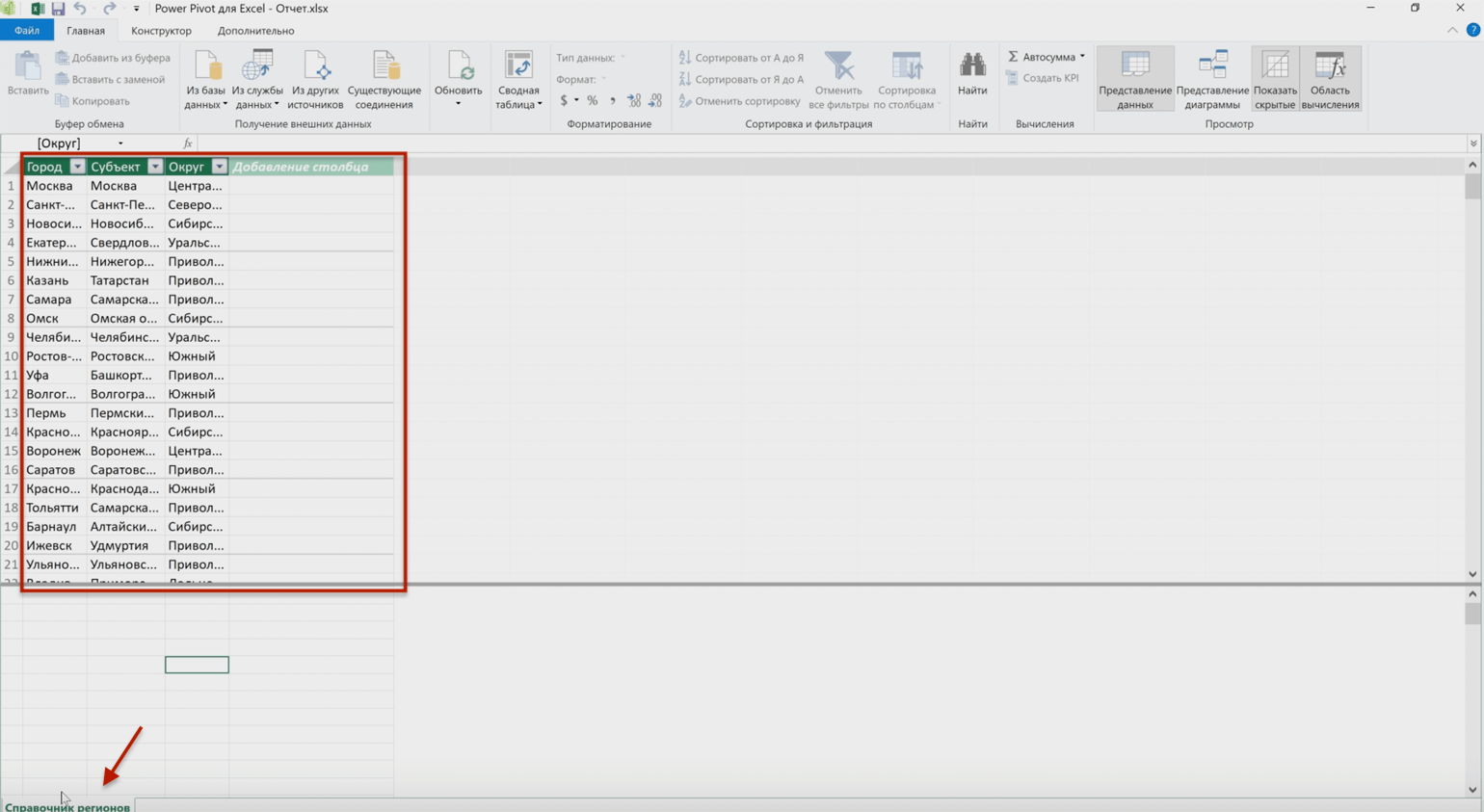
Готово — первые данные загрузились в Power Pivot. В окне появился отдельный лист «Справочник регионов», на нём отражена та же таблица, что была и во внешнем источнике.
Шаг 4
Выгружаем данные из текстового файла
На вкладке «Главная» нажимаем кнопку «Из других источников». В появившемся окне выбираем «Текстовый файл» и нажимаем «Далее».
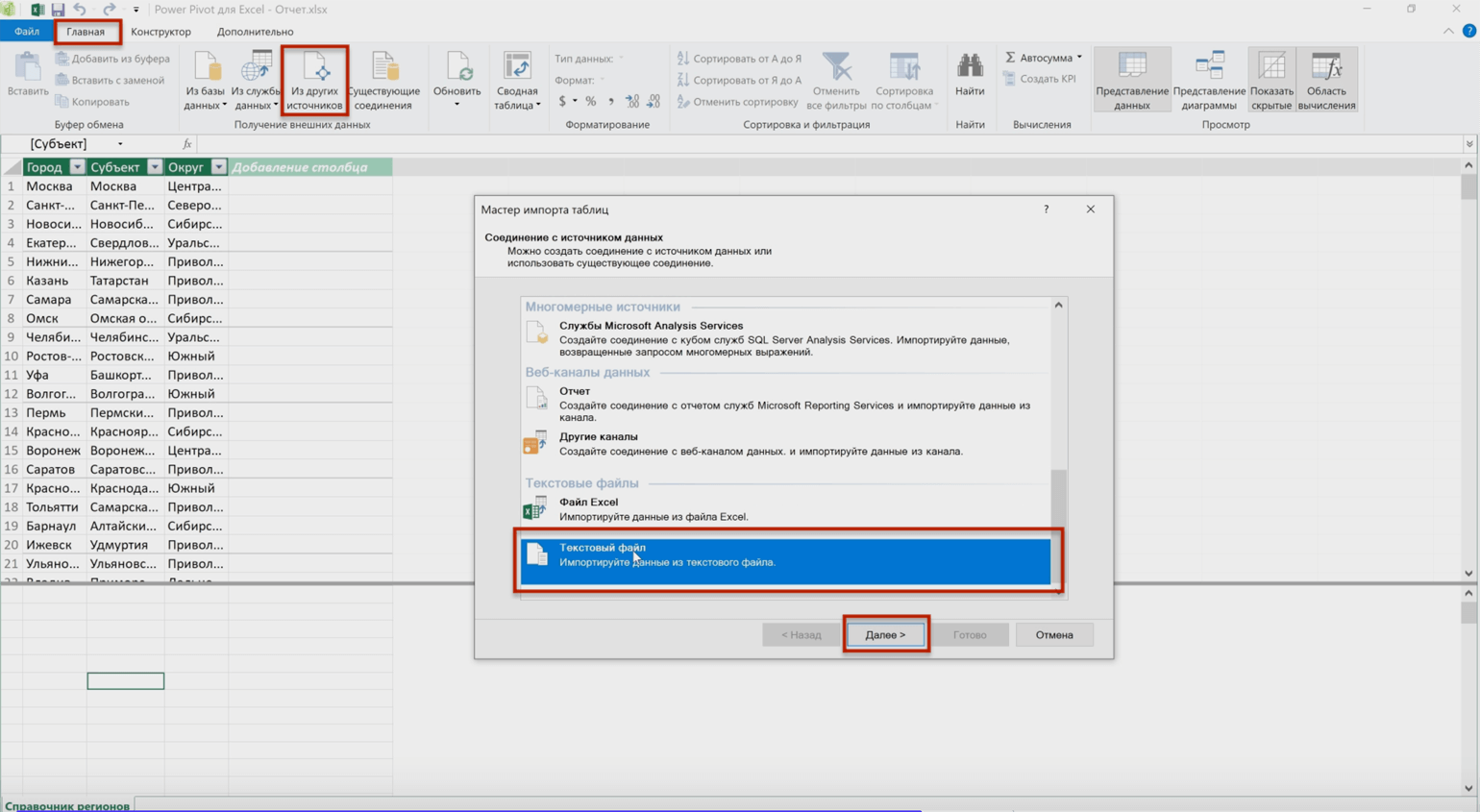
В появившемся окне в поле «Имя базы данных» прописываем адрес, где хранится текстовый файл с данными о продажах.
После этого в нижней части окна появляется предпросмотр таблицы из источника данных.
При необходимости корректируем настройки — например, меняем вид разделителя столбцов или отключаем ненужные графы таблицы. Затем нажимаем «Готово».
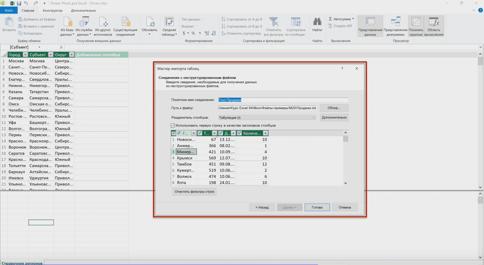
Начинается импорт выбранной таблицы из текстового файла в Power Pivot. После этого появляется окно с результатом. Проверяем информацию и нажимаем «Закрыть».
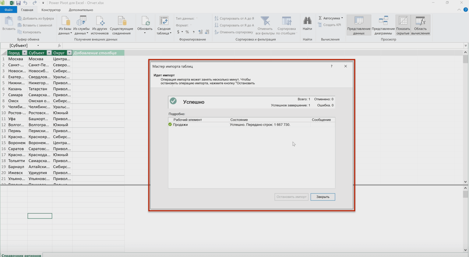
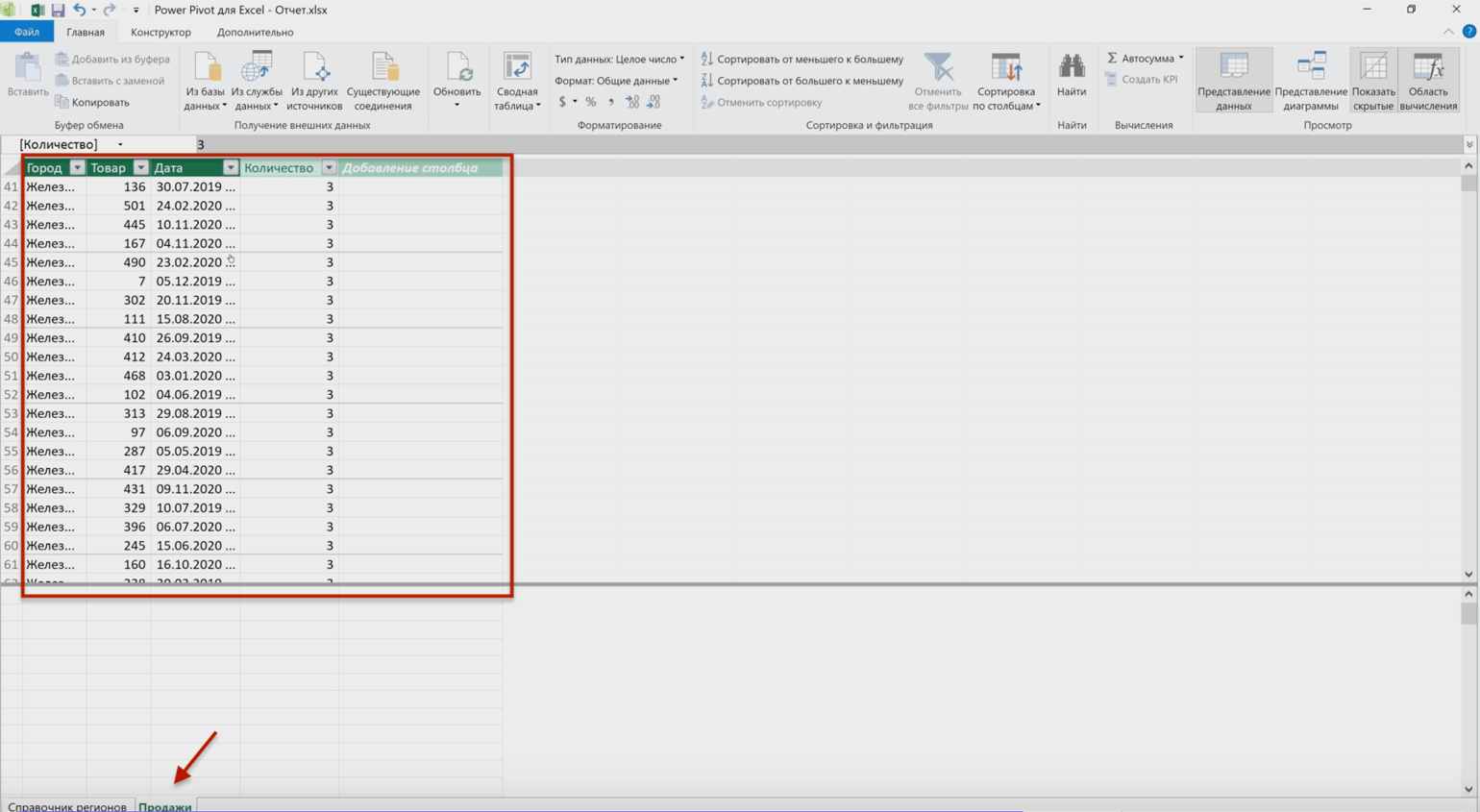
Готово — в окне Power Pivot появилась вторая вкладка «Продажи» — на ней более полутора миллионов строк. Напомним, в Excel без надстройки могло бы поместиться около миллиона.
Шаг 5
Выгружаем данные из файла Excel
По аналогии с предыдущим шагом на вкладке «Главная» нажимаем кнопку «Из других источников». Во всплывшем окне выбираем «Файл Excel» и нажимаем «Далее».
В появившемся окне в поле «Имя базы данных» прописываем адрес, по которому хранится файл Excel со справочником товаров. Нажимаем «Далее»,
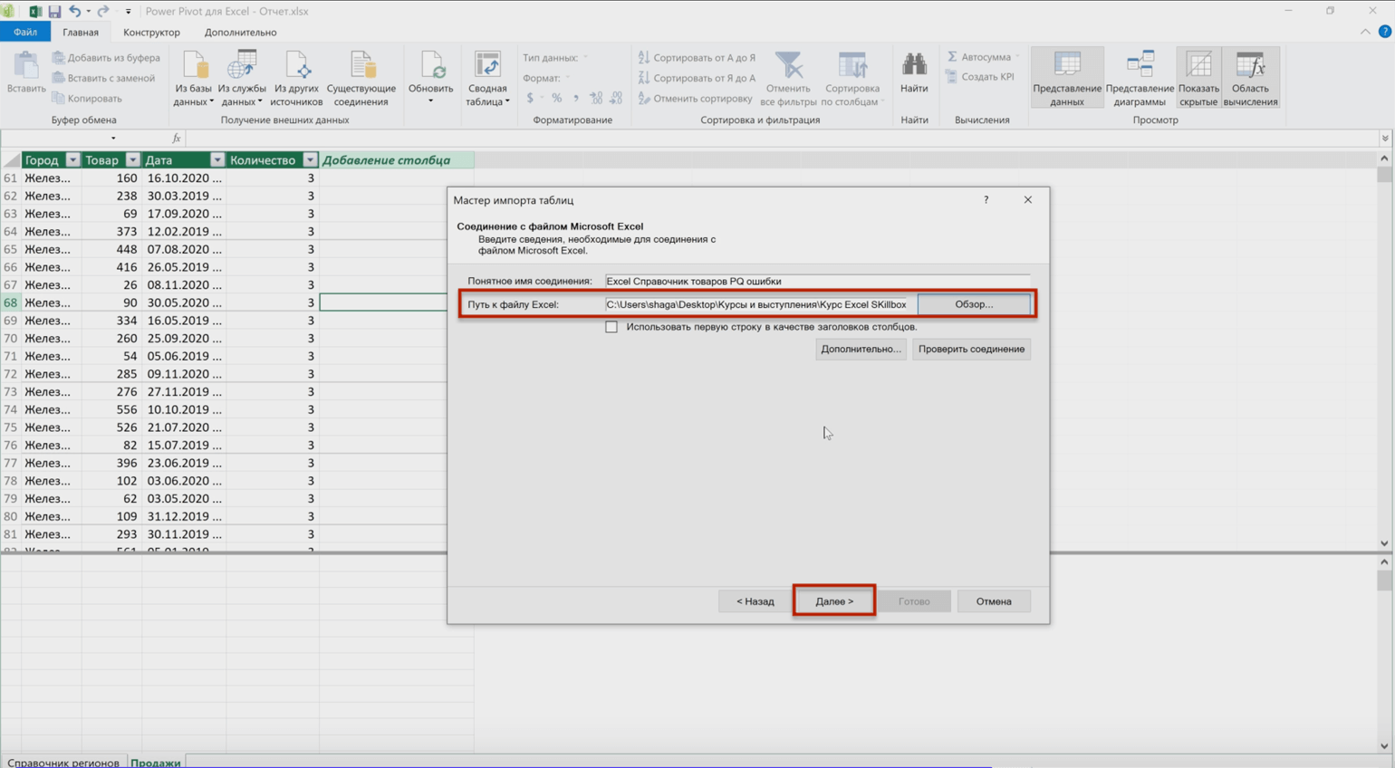
В следующем окне появляется список всех таблиц, которые хранятся в выбранной базе данных.
В нашем случае она одна — «Справочник товаров». Выбираем её и нажимаем «Готово».
Снова происходит импорт и появляется окно с результатом.
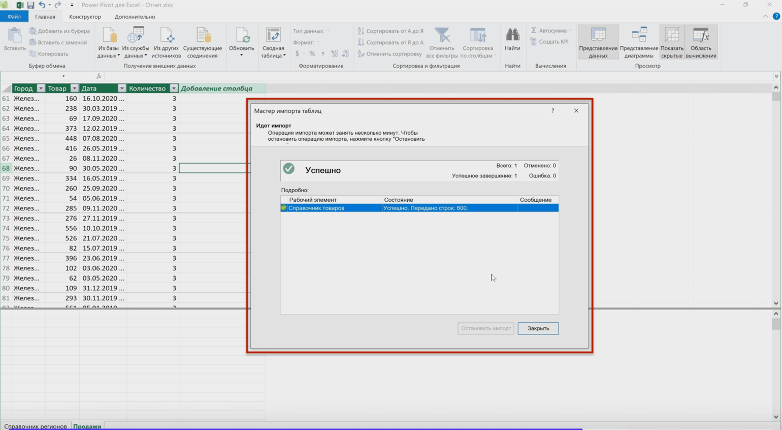
В окне Power Pivot появилась третья вкладка «Справочник товаров». Также со всеми данными, которые хранились в первоисточнике — внешнем файле Excel.
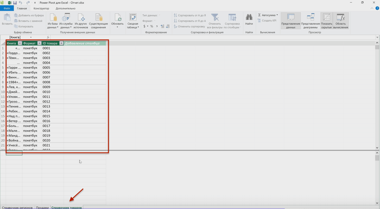
Шаг 6
Выгружаем данные из файла Power Point
В этом случае выгрузить данные можно только методом «копировать — вставить».
Открываем файл Power Point, содержащий ценовую политику. Выделяем таблицу, нажимаем правую кнопку мыши и выбираем «Скопировать».
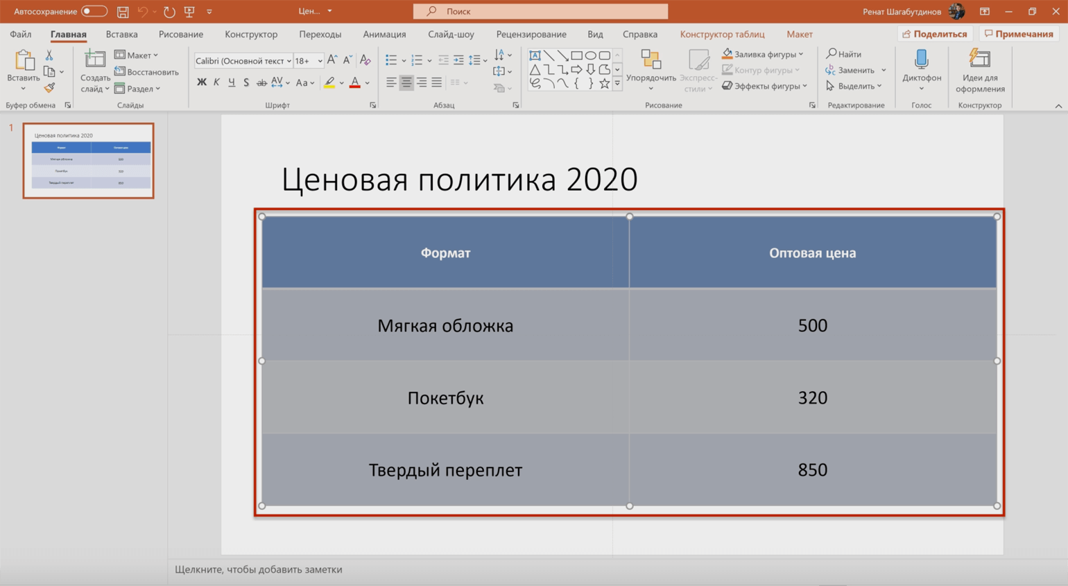
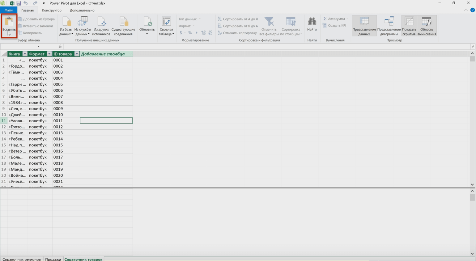
Затем возвращаемся в окно Power Pivot и на любой вкладке нажимаем кнопку «Вставить» на главной панели.
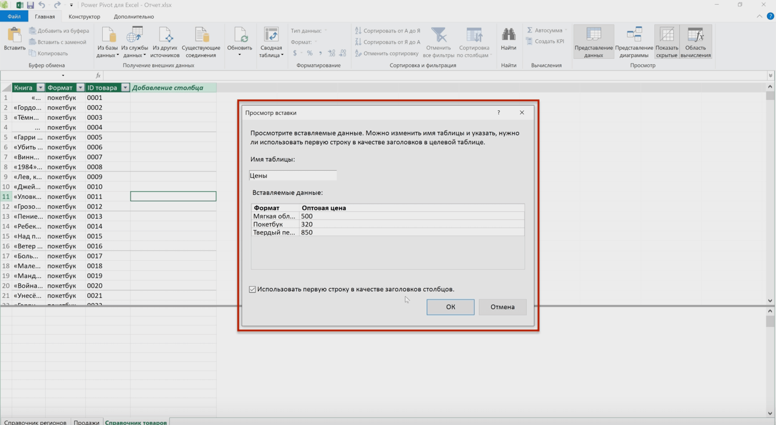
В появившемся окне вводим имя таблицы — «Цены» — и нажимаем «ОК».
Готово — в окне Power Pivot появилась четвёртая вкладка «Цены».
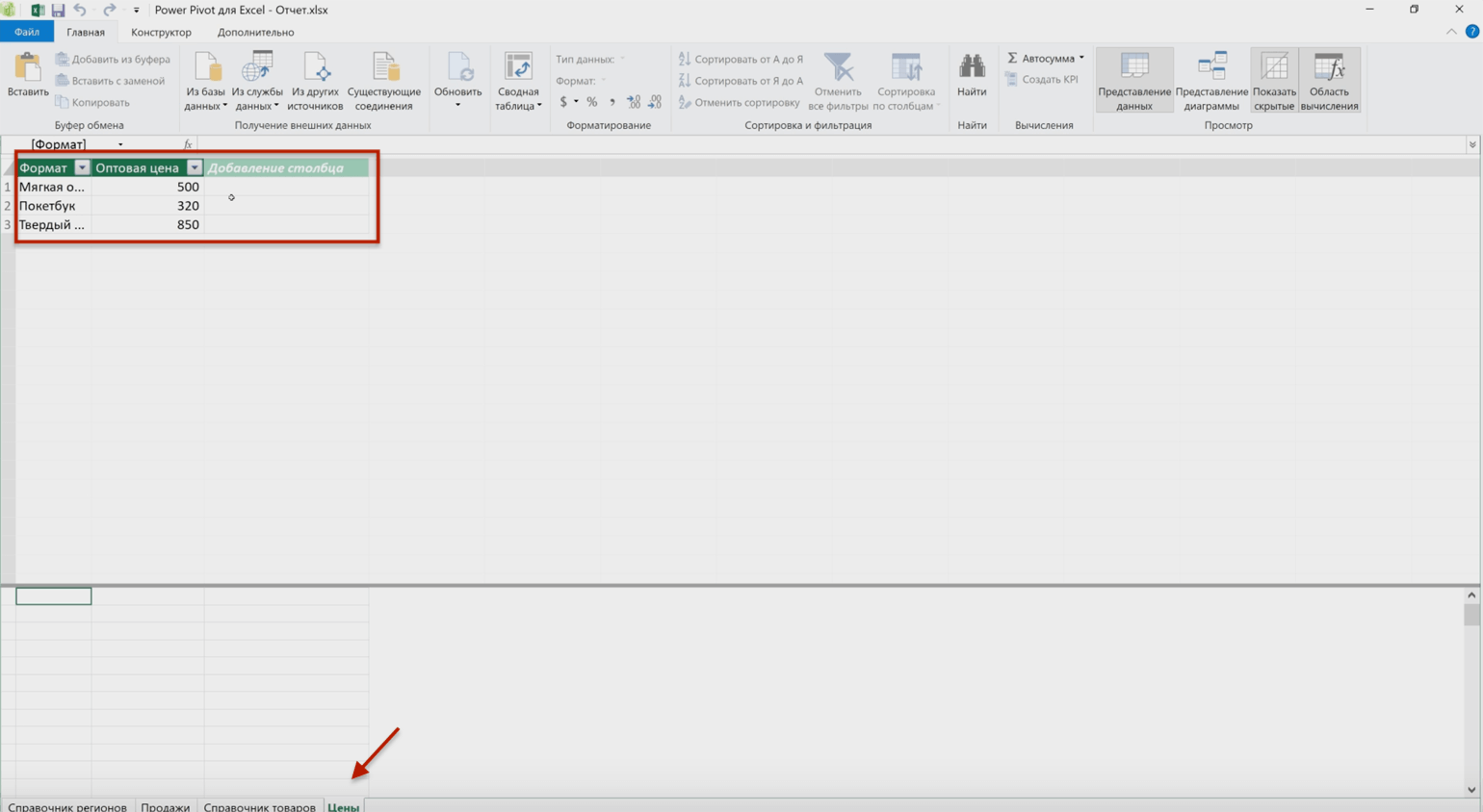
Важно понимать, что при таком варианте выгрузки данных — копировании и вставке — таблица не будет обновляться, если внести изменения в исходный файл Power Point.
В предыдущих трёх вариантах — при загрузке таблиц из базы данных, текстового файла и файла Excel — в случае изменения данных в исходных файлах они также изменятся и в Power Pivot. Ниже показываем, как это сделать.
Шаг 7
Обновляем данные из внешних источников в Power Pivot
Для этого на главной панели любой вкладки нужно нажать кнопку «Обновить», затем «Обновить все».
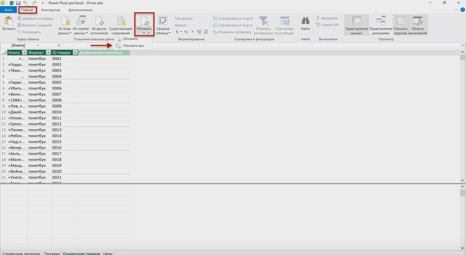
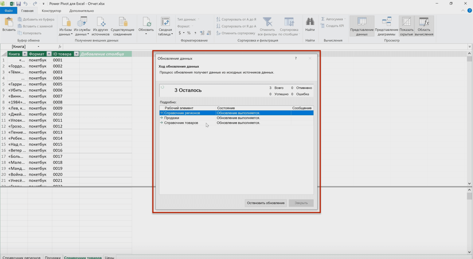
Появится окно, где будет видно, какие вкладки обновляются. В нашем случае это только первые три вкладки.
Обновление проходит быстро — примерно за 10–15 секунд обновляются три вкладки, в одной из которых более полутора миллионов строк.
Файл из Power Point придётся обновлять вручную.
Моделируем данные в Power Pivot
В предыдущем разделе мы загрузили данные из внешних источников в Power Pivot. Сейчас у нас есть четыре вкладки, в которых хранятся четыре таблицы: «Справочник регионов», «Продажи», «Справочник товаров», «Цены».
Задача этого этапа — связать данные всех таблиц так, чтобы можно было анализировать информацию одновременно по всем столбцам.
Шаг 1
Меняем режим представления данных в Power Pivot
Для этого на главной вкладке окна Power Pivot нажмём кнопку «Представление диаграммы».
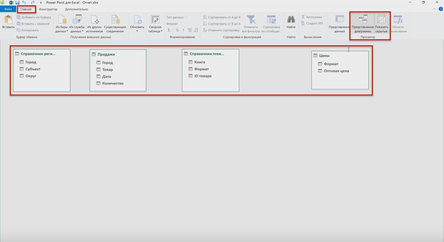
В этом режиме отображения каждая таблица показана в виде прямоугольника, в котором перечислены её столбцы. Для удобства эти прямоугольники можно двигать и менять местами.
В этом же режиме отображения в Power Pivot настраивают связи между таблицами.
Шаг 2
Настраиваем связи между данными таблиц
Первая связь. В таблице «Продажи» есть столбец «Город», но нет столбцов «Субъекты» и «Округ». Все эти столбцы, включая столбец «Город», есть в таблице «Справочник регионов».
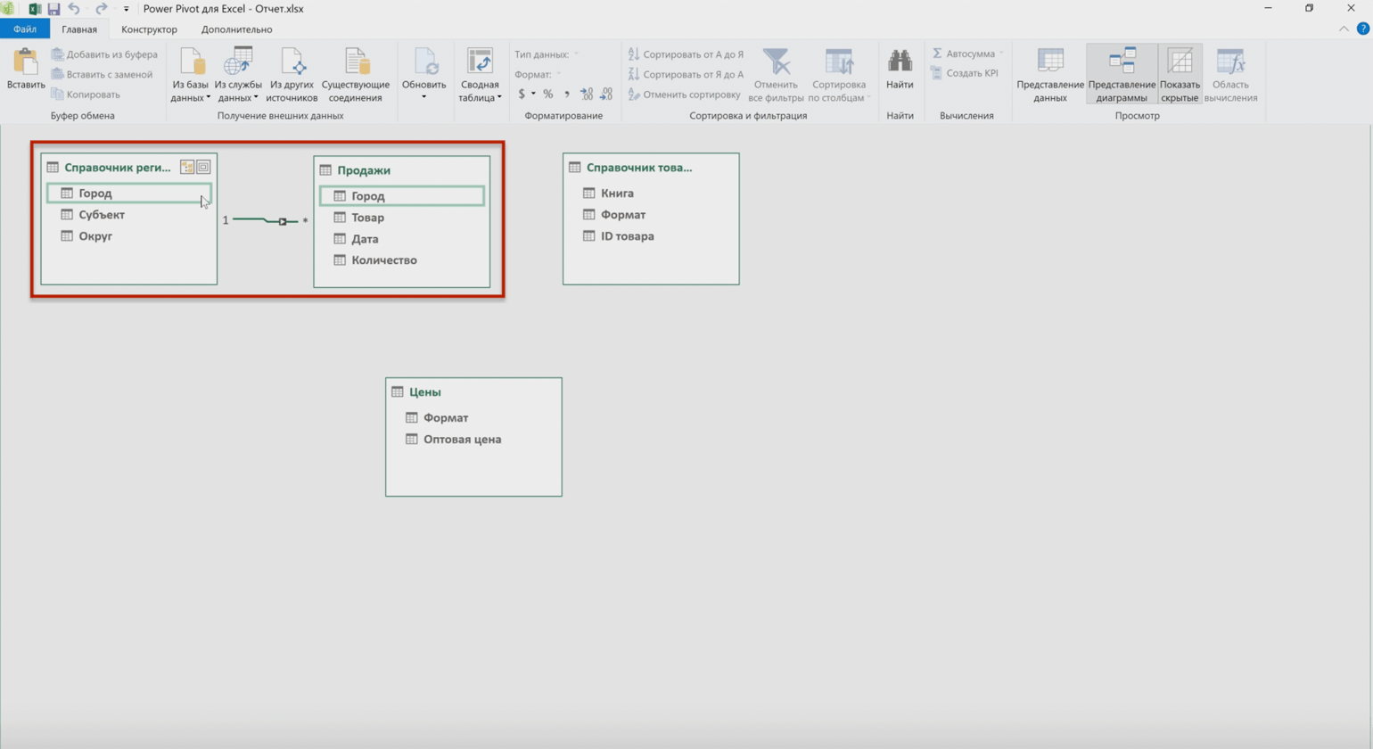
Соответственно, чтобы объединить данные этих двух таблиц, нужно создать связь по столбцу «Город». Для этого нужно зажать мышкой такой столбец в одной из таблиц и перетянуть его во вторую таблицу. Между таблицами появится линия.
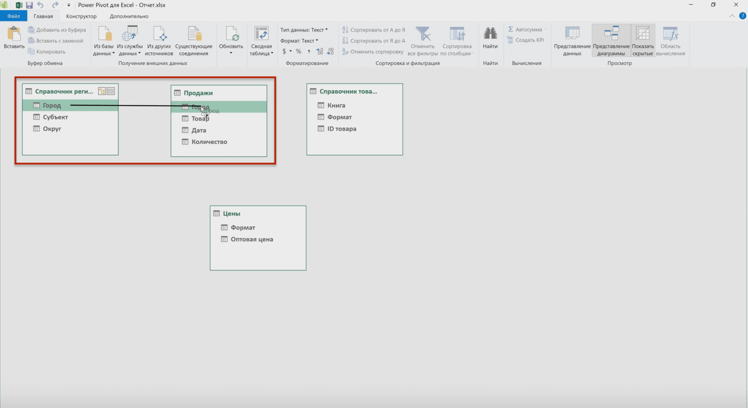
Готово — между таблицами «Справочник регионов» и «Продажи» появилась связь по столбцу «Город». Теперь у каждой строки продаж будет указан не только город, но также субъект и округ.
Вторая связь. В таблице «Продажи» есть столбец «Товар», где перечислены ID‑номера книг, но нет названий книг и их форматов. Все эти данные находятся в таблице «Справочник товаров».
По аналогии с предыдущей связью построим связь между столбцом «Товар» в таблице «Продажи» и столбцом «ID товара» в таблице «Справочник товаров».
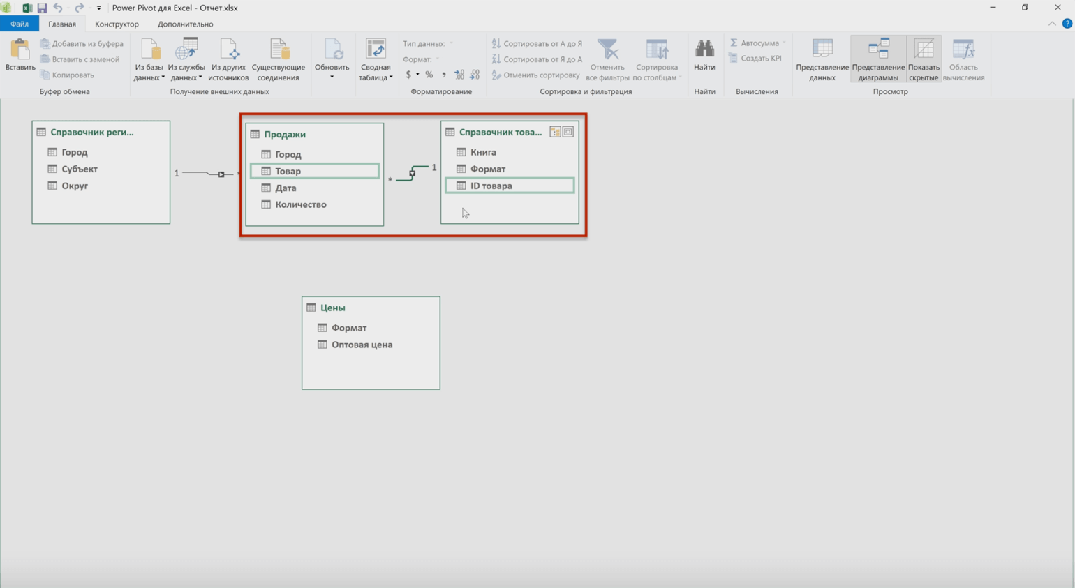
Названия столбцов, по которым строят связи между таблицами, не обязательно должны быть одинаковыми. Главное, чтобы в таких столбцах хранилась аналогичная информация. В нашем случае это ID-номера книг.
При этом Power Pivot не проверяет самостоятельно, правильно ли настроена связь — совпадают ли данные столбцов двух таблиц, — поэтому проводить связи между таблицами нужно внимательно.
Третья связь. Теперь к уже объединённым данным нужно добавить цены. Они хранятся в четвёртой таблице. Настроим связь между ней и таблицей «Справочник товаров» по столбцу «Формат».
Благодаря этой связи в «Справочнике товаров» появится информация о ценах на книги.
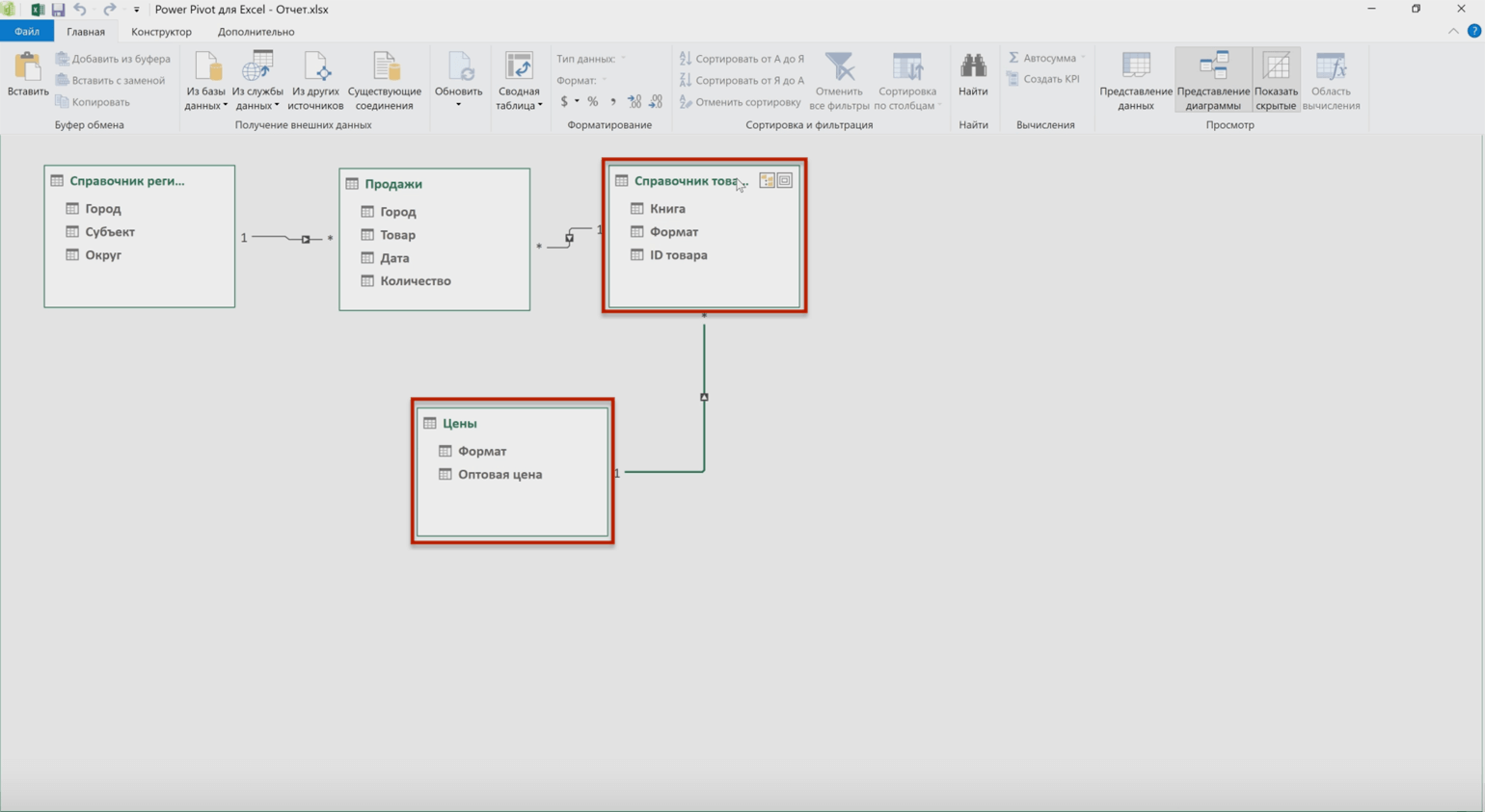
Готово. Мы построили модель из четырёх таблиц из разных источников и связали данные этих таблиц по идентичным столбцам. Чтобы увидеть результат, нужно создать сводную таблицу.
Шаг 3
Создаём сводную таблицу.
На главной вкладке нажимаем кнопку «Сводная таблица».
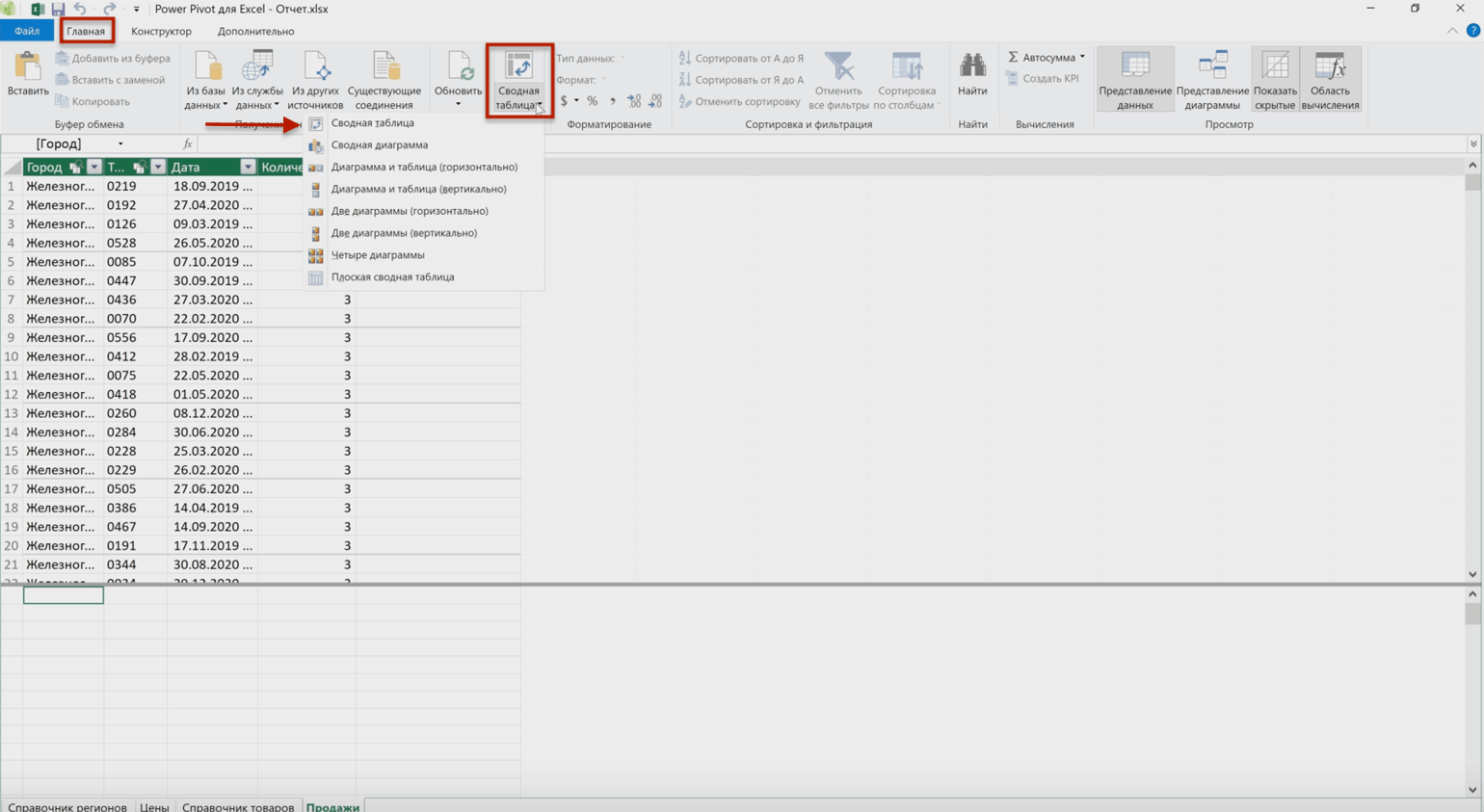
Дальше выбираем, на каком листе нужно создать сводную таблицу — на новом или на существующем.
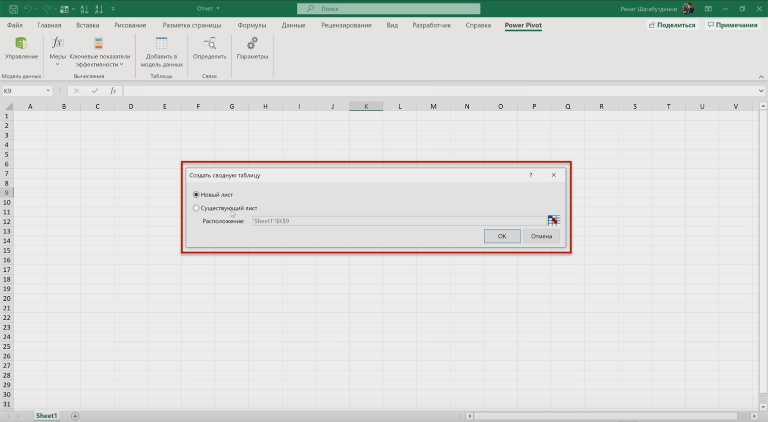
Готово — появился новый лист для сводной таблицы. Слева на листе расположена область, где появится отчёт сводной таблицы после настроек. Справа — панель «Поля сводной таблицы», в которой мы будем работать с этими настройками.
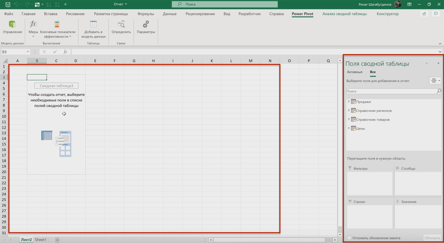
Панель «Поля сводной таблицы» состоит из двух частей. В верхней части находится список полей — в нашем случае Power Pivot перенёс в список полей данные четырёх таблиц, которые мы связали между собой. В нижней части — четыре области: «Значения», «Строки», «Столбцы» и «Фильтры». У каждой области своё назначение.
Чтобы создать отчёт сводной таблицы, нужно выбрать необходимые поля из списка полей и перенести их в нужную область.
Подробнее о назначении областей, а также о том, как строить и настраивать сводные таблицы в стандартной версии Excel, говорили в этой статье Skillbox Media.
Для примера построим отчёт в форме сводной таблицы, который покажет количество продаж издательства в субъектах России с детализацией по формату книг.
Для этого в область «Строки» перенесём поля «Округ» и «Субъект» из «Справочника регионов», в область «Значения» — поле «Количество» из таблицы «Продажи», в область «Столбцы» — поле «Формат» из «Справочника товаров».
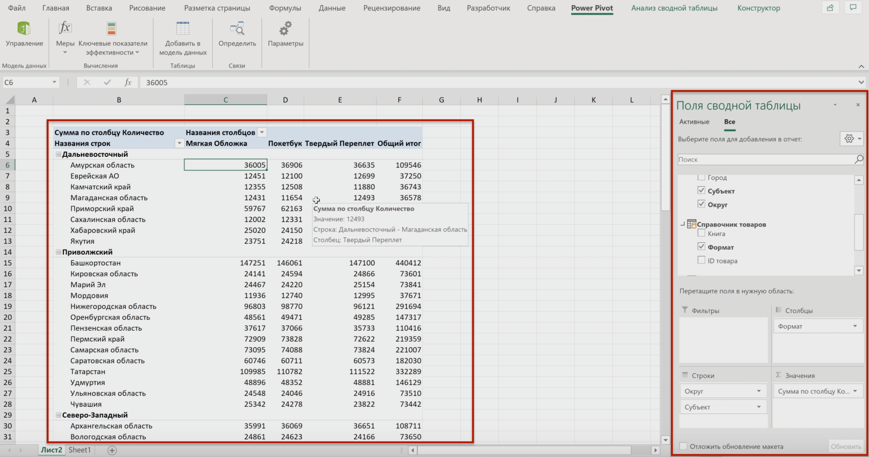
Готово. Мы получили таблицу, где по вертикали расположены все субъекты и округа страны, по горизонтали — количество проданных книг с разбивкой по форматам.
По такому же принципу можно строить другие отчёты — в зависимости от того, какую информацию для анализа нужно получить. Например, в отчёте можно показать количество продаж с детализацией по названиям книг и датам их продажи.
Как узнать больше о работе в Excel
- В этой статье Skillbox Media собрали в одном месте 15 статей и видео об инструментах Excel, которые ускорят и упростят работу с электронными таблицами.
- В Skillbox есть курс «Excel + Google Таблицы с нуля до PRO». Он подойдёт как новичкам, которые хотят научиться работать в Excel с нуля, так и уверенным пользователям, которые хотят улучшить свои навыки. На курсе учат быстро делать сложные расчёты, визуализировать данные, строить прогнозы, работать с внешними источниками данных, создавать макросы и скрипты.
- Кроме того, Skillbox даёт бесплатный доступ к записи онлайн-интенсива «Экспресс-курс по Excel: осваиваем таблицы с нуля за 3 дня». Он подходит для начинающих пользователей. На нём можно научиться создавать и оформлять листы, вводить данные, использовать формулы и функции для базовых вычислений, настраивать пользовательские форматы и создавать формулы с абсолютными и относительными ссылками.
Другие материалы Skillbox Media по Excel
- Как сделать сводные таблицы в Excel: пошаговая инструкция со скриншотами
- Как сделать ВПР в Excel: пошаговая инструкция со скриншотами
- Основы Excel: работаем с выпадающим списком. Пошаговая инструкция со скриншотами
- Как сделать сортировку в Excel: детальная инструкция со скриншотами
- Как установить фильтр и расширенный фильтр в Excel: детальные инструкции со скриншотами
- Для чего нужны макросы в Excel и как их сделать: инструкция со скриншотами